Mathematical Modeling 4 1 Introduction 4 2 Modeling

数学建模 Mathematical Modeling

第四讲 差分方程模型 4. 1 Introduction 4. 2 Modeling with a Difference Equation 4. 2. 1 An Investment Annuity 4. 2. 2 Growth of a Yeast Culture 4. 3 Modeling with Difference Equations 4. 3. 1 Travelers' Tendencies at a Regional Airport 4. 3. 2 Spider web model of the market 4. 3. 3 Competitive Hunter Model 4. 3. 4 Retarding growth model of the population 2

4. 1 Introduction

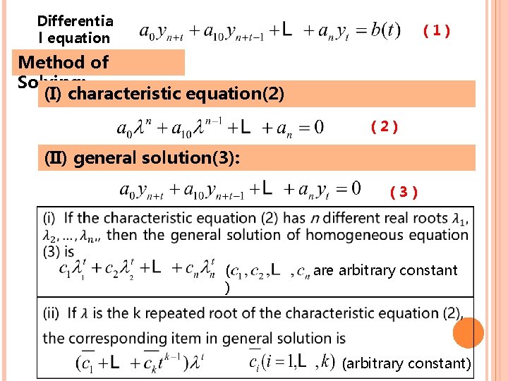
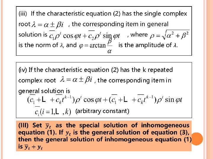
Differentia l equation （1） Method of Solving: (I) characteristic equation(2) （2） (II) general solution(3): （3） ( ) are arbitrary constant (arbitrary constant)

(iv) If the characteristic equation (2) has the k repeated complex root , the corresponding item in general solution is (arbitrary constant)

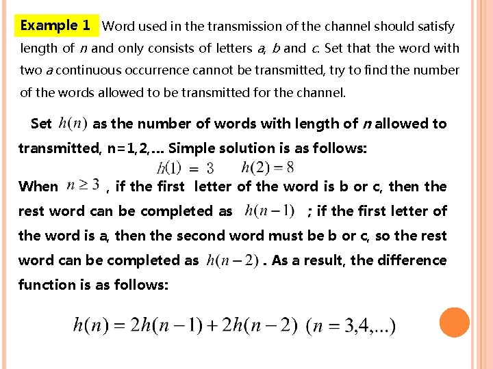
Example 1 Word used in the transmission of the channel should satisfy length of n and only consists of letters a, b and c. Set that the word with two a continuous occurrence cannot be transmitted, try to find the number of the words allowed to be transmitted for the channel. Set as the number of words with length of n allowed to transmitted, n=1, 2, … Simple solution is as follows: When , if the first letter of the word is b or c, then the rest word can be completed as ; if the first letter of the word is a, then the second word must be b or c, so the rest word can be completed as function is as follows: . As a result, the difference

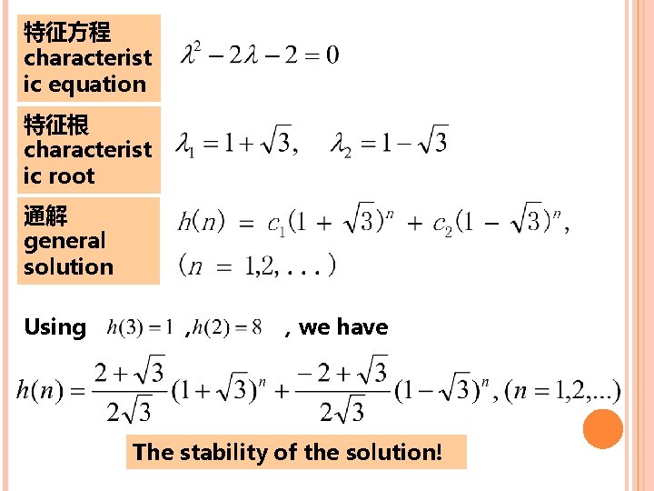
特征方程 characterist ic equation 特征根 characterist ic root 通解 general solution Using ， ，we have The stability of the solution!

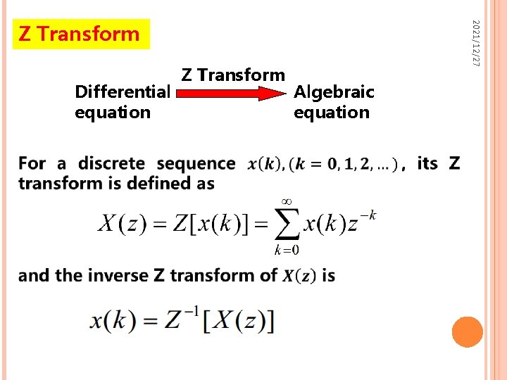
2021/12/27 Z Transform Differential equation Z Transform Algebraic equation

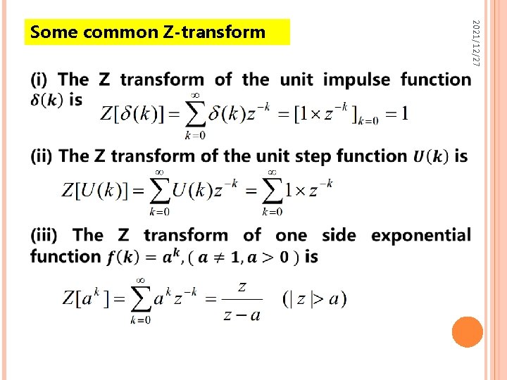
2021/12/27 Some common Z-transform

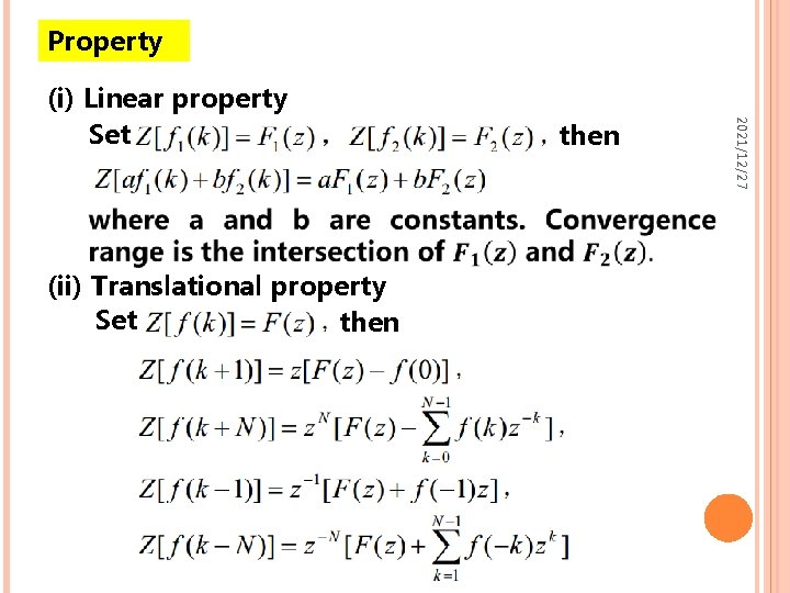
Property (ii) Translational property Set then 2021/12/27 (i) Linear property Set

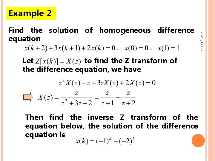
Example 2 Let to find the Z transform of the difference equation, we have Then find the inverse Z transform of the equation below, the solution of the difference equation is 2021/12/27 Find the solution of homogeneous difference equation

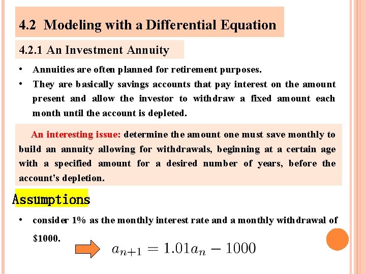
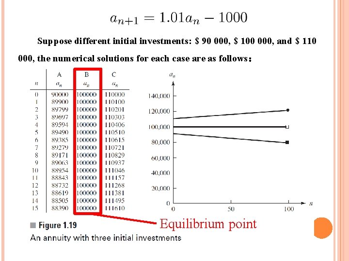
4. 2 Modeling with a Differential Equation 4. 2. 1 An Investment Annuity • Annuities are often planned for retirement purposes. • They are basically savings accounts that pay interest on the amount present and allow the investor to withdraw a fixed amount each month until the account is depleted. An interesting issue: determine the amount one must save monthly to build an annuity allowing for withdrawals, beginning at a certain age with a specified amount for a desired number of years, before the account's depletion. Assumptions • consider 1% as the monthly interest rate and a monthly withdrawal of $1000.

Suppose different initial investments: $ 90 000, $ 100 000, and $ 110 000, the numerical solutions for each case are as follows： Equilibrium point

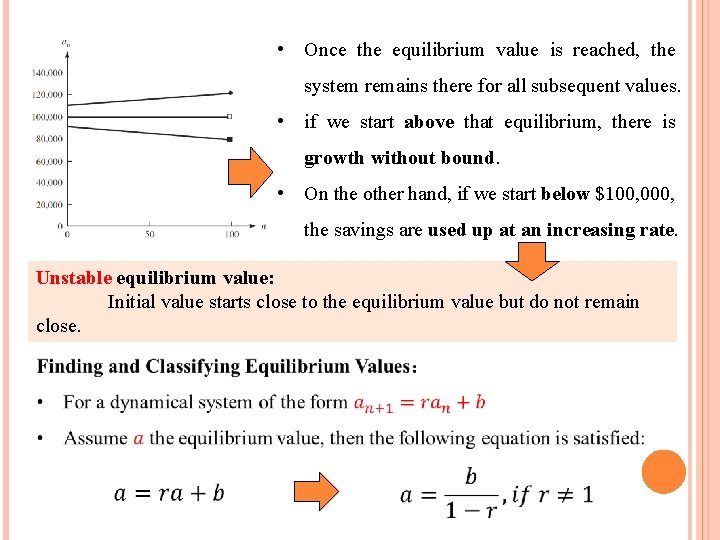
• Once the equilibrium value is reached, the system remains there for all subsequent values. • if we start above that equilibrium, there is growth without bound. • On the other hand, if we start below $100, 000, the savings are used up at an increasing rate. Unstable equilibrium value: Initial value starts close to the equilibrium value but do not remain close.

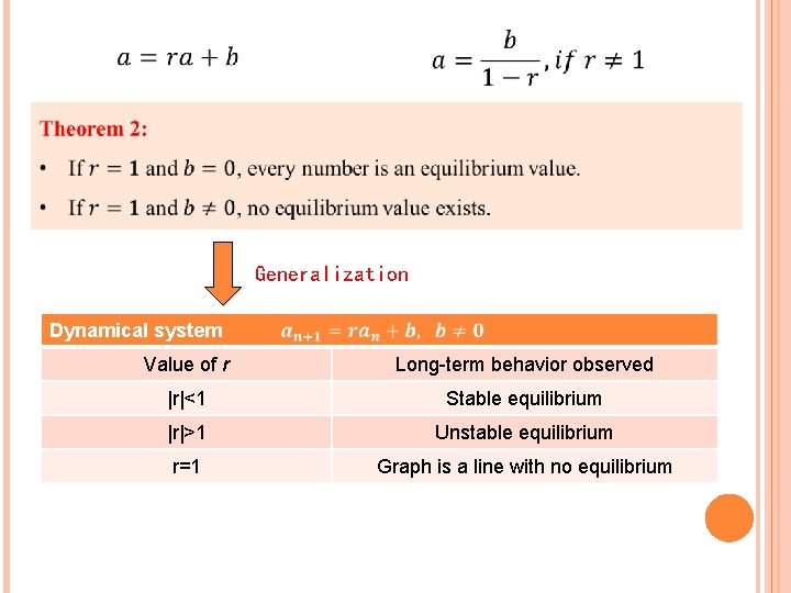
Generalization Dynamical system Value of r Long-term behavior observed |r|<1 Stable equilibrium |r|>1 Unstable equilibrium r=1 Graph is a line with no equilibrium

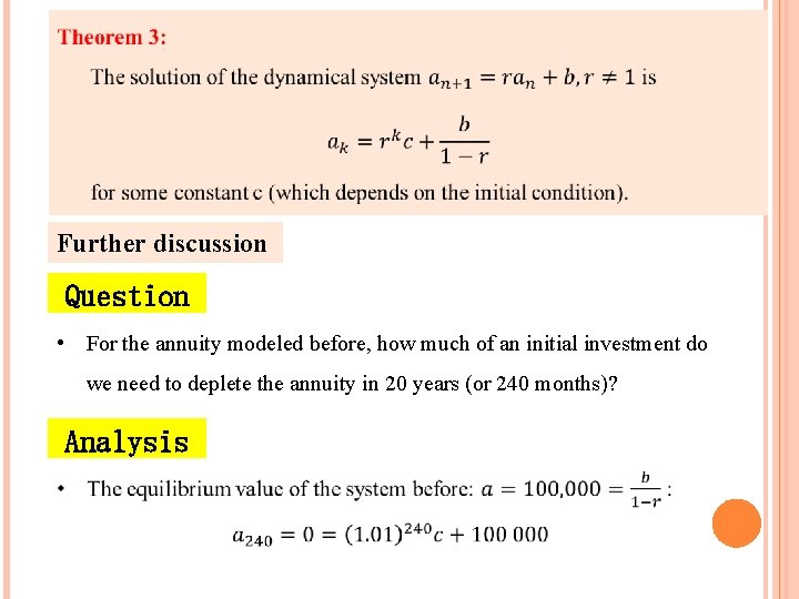
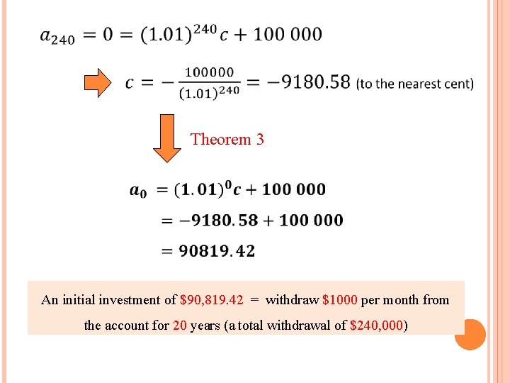
Further discussion Question • For the annuity modeled before, how much of an initial investment do we need to deplete the annuity in 20 years (or 240 months)? Analysis

Theorem 3 An initial investment of $90, 819. 42 = withdraw $1000 per month from the account for 20 years (a total withdrawal of $240, 000)

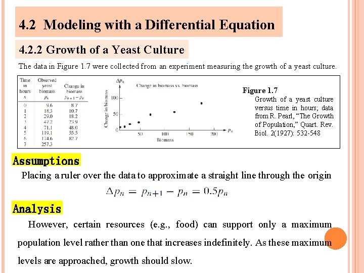
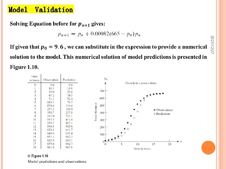
4. 2 Modeling with a Differential Equation 4. 2. 2 Growth of a Yeast Culture The data in Figure 1. 7 were collected from an experiment measuring the growth of a yeast culture. Figure 1. 7 Growth of a yeast culture versus time in hours; data from R. Pearl, “The Growth of Population, ” Quart. Rev. Biol. 2(1927): 532 -548 Assumptions Placing a ruler over the data to approximate a straight line through the origin Analysis However, certain resources (e. g. , food) can support only a maximum population level rather than one that increases indefinitely. As these maximum levels are approached, growth should slow.

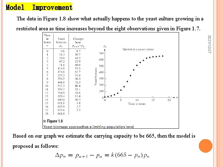
Model Improvement The data in Figure 1. 8 show what actually happens to the yeast culture growing in a restricted area as time increases beyond the eight observations given in Figure 1. 7. 2021/12/27 Based on our graph we estimate the carrying capacity to be 665, then the model is proposed as follows:

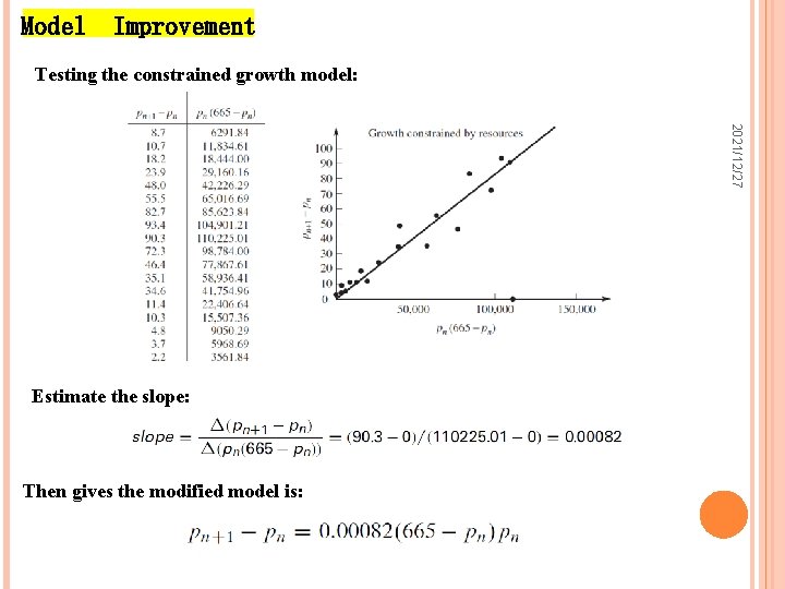
Model Improvement Testing the constrained growth model: 2021/12/27 Estimate the slope: Then gives the modified model is:

Model Validation 2021/12/27

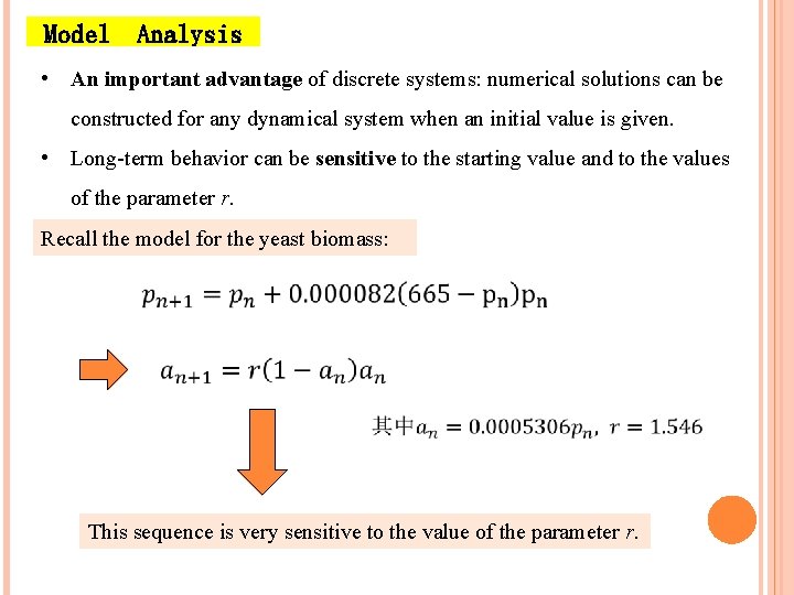
Model Analysis • An important advantage of discrete systems: numerical solutions can be constructed for any dynamical system when an initial value is given. • Long-term behavior can be sensitive to the starting value and to the values of the parameter r. Recall the model for the yeast biomass: This sequence is very sensitive to the value of the parameter r.

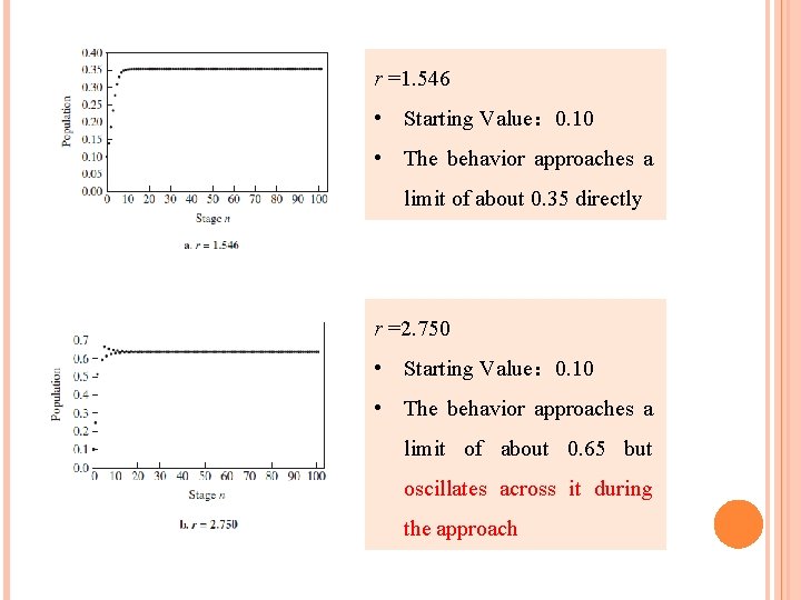
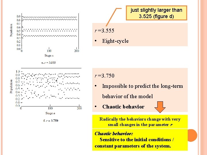
r =1. 546 • Starting Value： 0. 10 • The behavior approaches a limit of about 0. 35 directly r =2. 750 • Starting Value： 0. 10 • The behavior approaches a limit of about 0. 65 but oscillates across it during the approach

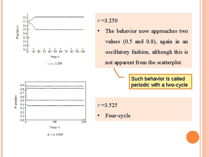
r =3. 250 • The behavior now approaches two values (0. 5 and 0. 8), again in an oscillatory fashion, although this is not apparent from the scatterplot. Such behavior is called periodic with a two-cycle r =3. 525 • Four-cycle

just slightly larger than 3. 525 (figure d) r =3. 555 • Eight-cycle r =3. 750 • Impossible to predict the long-term behavior of the model • Chaotic behavior Radically the behaviors change with very small changes in the parameter r Chaotic behavior: Sensitive to the initial conditions / constant parameters of the system.

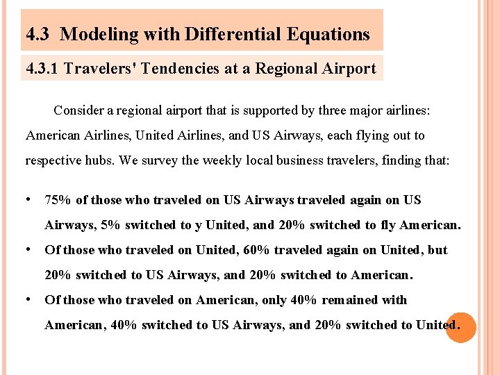
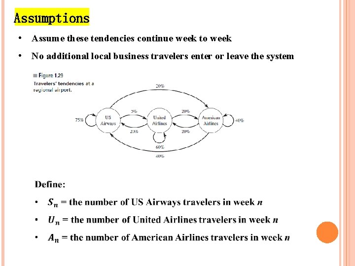
4. 3 Modeling with Differential Equations 4. 3. 1 Travelers' Tendencies at a Regional Airport Consider a regional airport that is supported by three major airlines: American Airlines, United Airlines, and US Airways, each flying out to respective hubs. We survey the weekly local business travelers, finding that: • 75% of those who traveled on US Airways traveled again on US Airways, 5% switched to y United, and 20% switched to fly American. • Of those who traveled on United, 60% traveled again on United, but 20% switched to US Airways, and 20% switched to American. • Of those who traveled on American, only 40% remained with American, 40% switched to US Airways, and 20% switched to United.

Assumptions • Assume these tendencies continue week to week • No additional local business travelers enter or leave the system

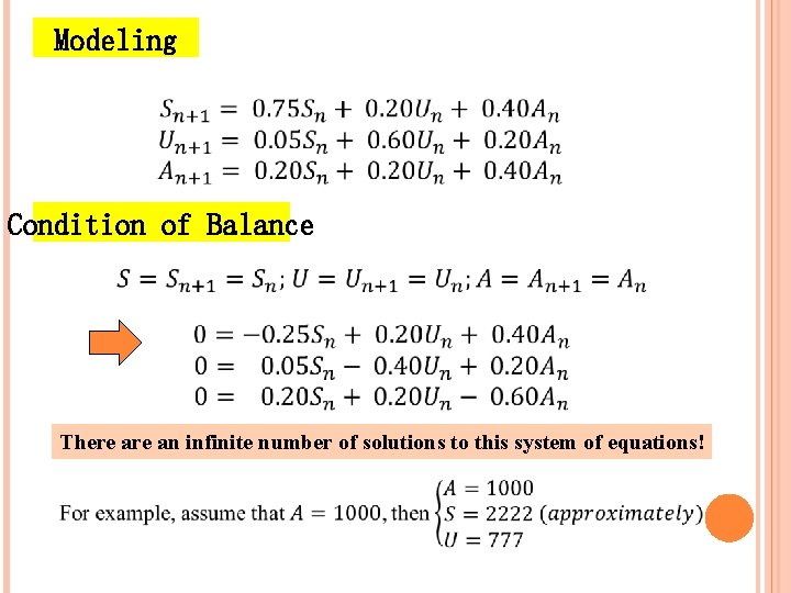
Modeling Condition of Balance There an infinite number of solutions to this system of equations!

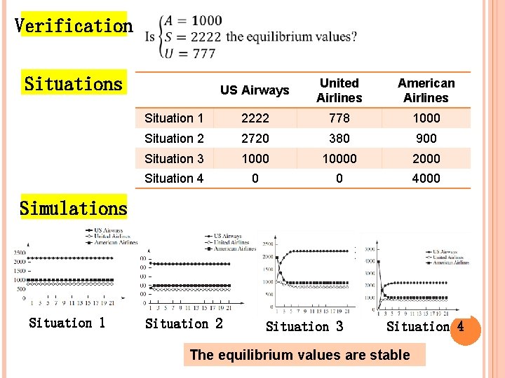
Verification Situations US Airways United Airlines American Airlines Situation 1 2222 778 1000 Situation 2 2720 380 900 Situation 3 10000 2000 Situation 4 0 0 4000 Simulations Situation 1 Situation 2 Situation 3 Situation 4 The equilibrium values are stable

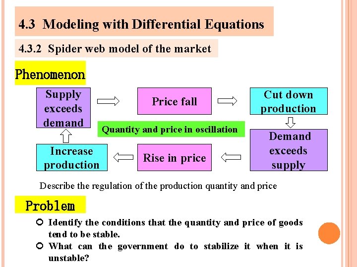
4. 3 Modeling with Differential Equations 4. 3. 2 Spider web model of the market Phenomenon Supply exceeds demand Increase production Price fall Quantity and price in oscillation Rise in price Cut down production Demand exceeds supply Describe the regulation of the production quantity and price Problem Identify the conditions that the quantity and price of goods tend to be stable. What can the government do to stabilize it when it is unstable?

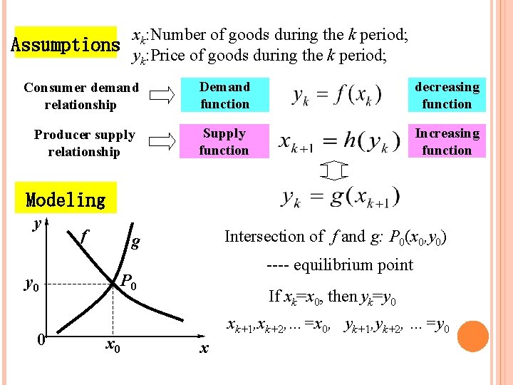
xk: Number of goods during the k period; Assumptions y : Price of goods during the k period; k Consumer demand relationship Demand function decreasing function Producer supply relationship Supply function Increasing function Modeling y y 0 0 f Intersection of f and g: P 0(x 0, y 0) g ---- equilibrium point P 0 x 0 If xk=x 0, then yk=y 0 xk+1, xk+2, …=x 0, yk+1, yk+2, …=y 0 x

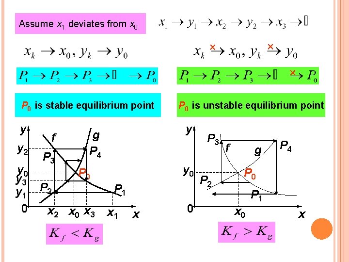
Assume x 1 deviates from x 0 P 0 is stable equilibrium point y y 2 y 0 y 3 y 1 0 f P 3 P 2 y g P 4 y 0 P 0 x 2 x 0 x 3 P 0 is unstable equilibrium point P 1 x 0 P 3 P 2 f g P 4 P 0 P 1 x 0 x

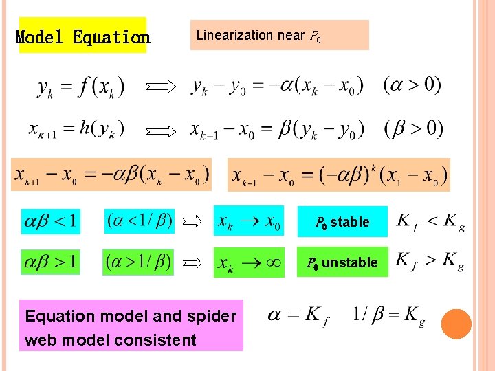
Model Equation Linearization near P 0 stable P 0 unstable Equation model and spider web model consistent

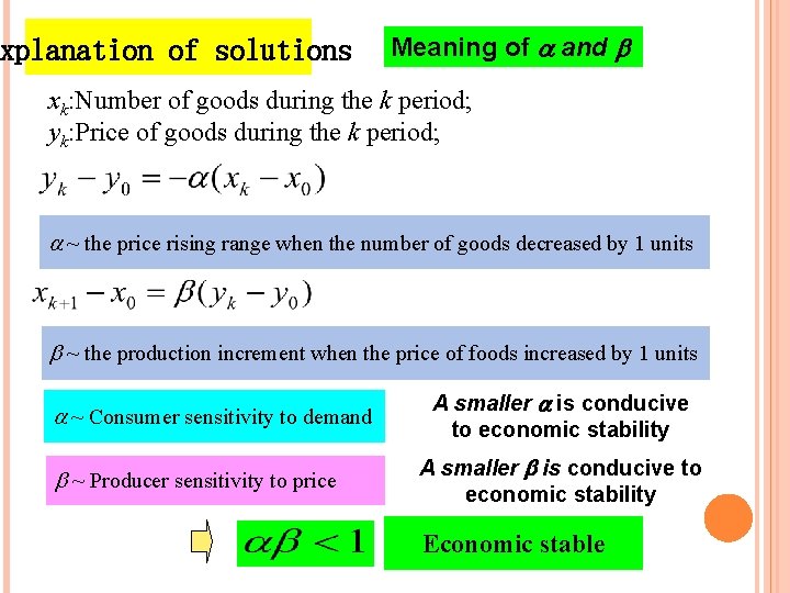
xplanation of solutions Meaning of and xk: Number of goods during the k period; yk: Price of goods during the k period; ~ the price rising range when the number of goods decreased by 1 units ~ the production increment when the price of foods increased by 1 units ~ Consumer sensitivity to demand ~ Producer sensitivity to price A smaller is conducive to economic stability Economic stable

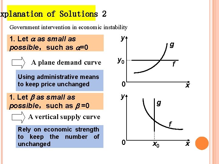
Explanation of Solutions 2 Government intervention in economic instability 1. Let as small as possible，such as =0 A plane demand curve Using administrative means to keep price unchanged 1. Let as small as possible，such as =0 A vertical supply curve Rely on economic strength to keep the number of unchanged y g y 0 f 0 y x g f 0 x

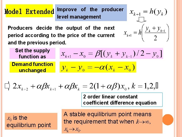
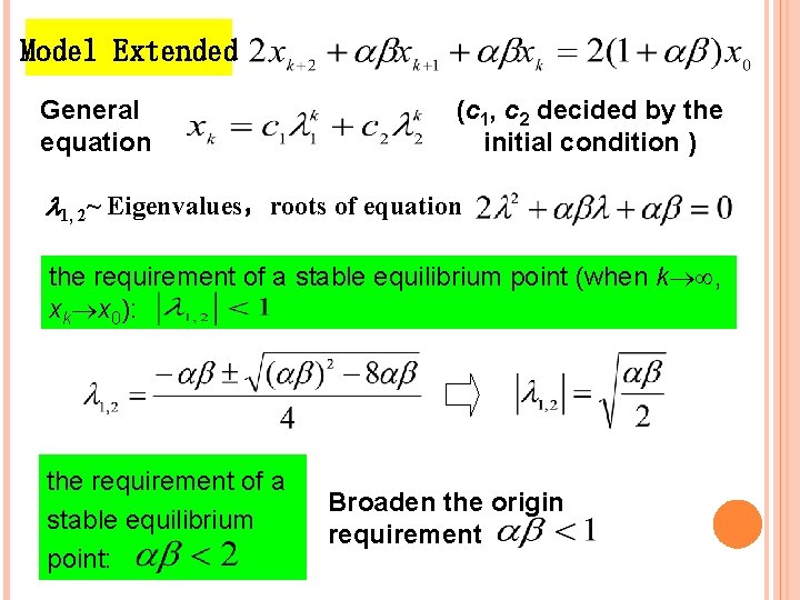
Model Extended Improve of the producer level management Producers decide the output of the next period according to the price of the current and the previous period. Set the supply function as Demand function unchanged 2 order linear constant coefficient difference equation x 0 is the equilibrium point A stable equilibrium point means the requirement that when k , xk x 0.

Model Extended General equation (c 1, c 2 decided by the initial condition ) 1, 2~ Eigenvalues，roots of equation the requirement of a stable equilibrium point (when k , xk x 0): the requirement of a stable equilibrium point: Broaden the origin requirement

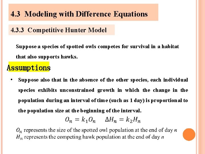
4. 3 Modeling with Difference Equations 4. 3. 3 Competitive Hunter Model Suppose a species of spotted owls competes for survival in a habitat that also supports hawks. Assumptions • Suppose also that in the absence of the other species, each individual species exhibits unconstrained growth in which the change in the population during an interval of time (such as 1 day) is proportional to the population size at the beginning of the interval.

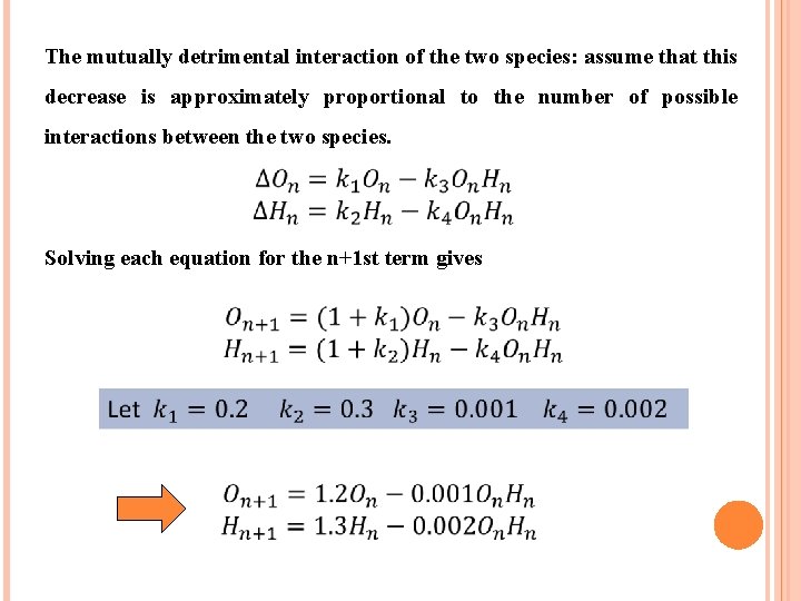
The mutually detrimental interaction of the two species: assume that this decrease is approximately proportional to the number of possible interactions between the two species. Solving each equation for the n+1 st term gives

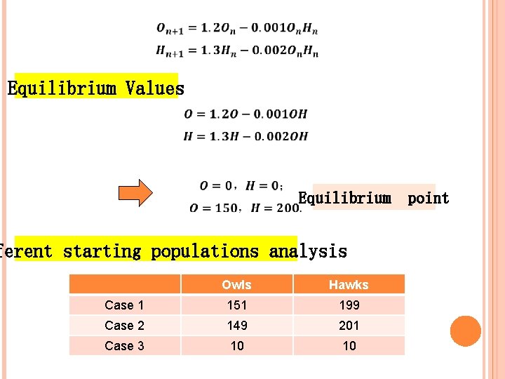
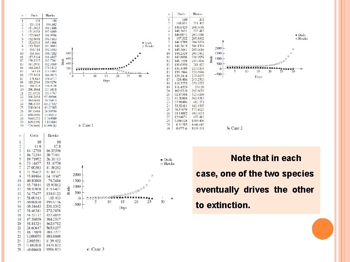
Equilibrium Values Equilibrium point ferent starting populations analysis Owls Hawks Case 1 151 199 Case 2 149 201 Case 3 10 10

Note that in each case, one of the two species eventually drives the other to extinction.

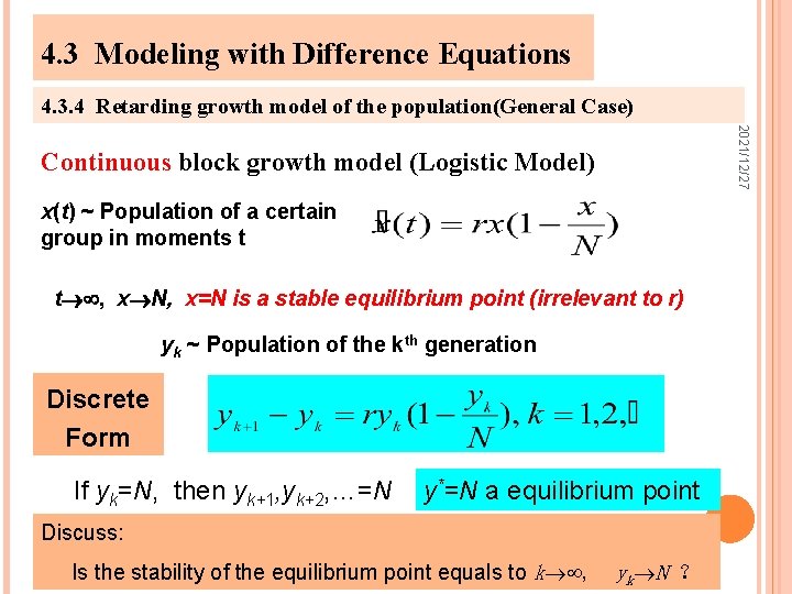
4. 3 Modeling with Difference Equations 4. 3. 4 Retarding growth model of the population(General Case) x(t) ~ Population of a certain group in moments t t , x N, x=N is a stable equilibrium point (irrelevant to r) yk ~ Population of the kth generation Discrete Form If yk=N, then yk+1, yk+2, …=N y*=N a equilibrium point Discuss: Is the stability of the equilibrium point equals to k , yk N ？ 2021/12/27 Continuous block growth model (Logistic Model)

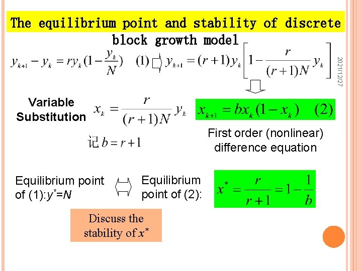
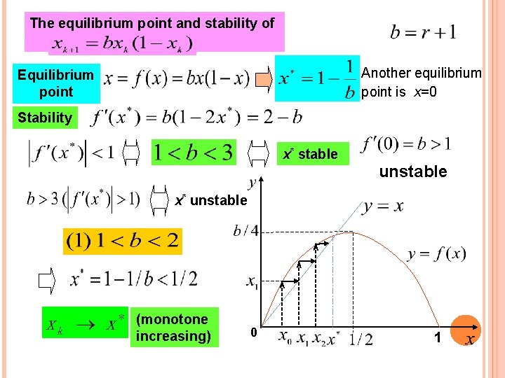
The equilibrium point and stability of discrete block growth model 2021/12/27 Variable Substitution First order (nonlinear) difference equation Equilibrium point of (1): y*=N Equilibrium point of (2): Discuss the stability of x*

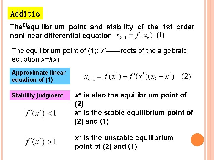
Additio The nequilibrium point and stability of the 1 st order nonlinear differential equation The equilibrium point of (1): x*——roots of the algebraic equation x=f(x) Approximate linear equation of (1) Stability judgment x* is also the equilibrium point of (2) x* is the stable equilibrium point of (2) and (1) x* is the unstable equilibrium point of (2) and (1)

The equilibrium point and stability of Another equilibrium point is x=0 Equilibrium point Stability x* stable unstable x* unstable (monotone increasing) 0 1

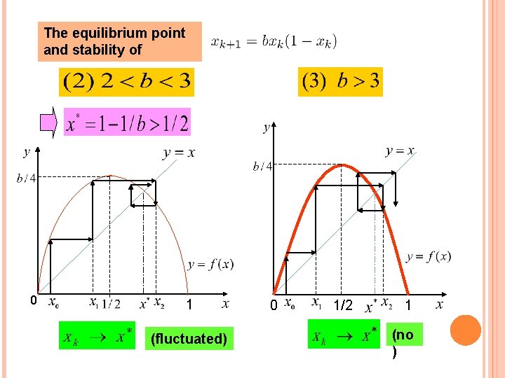
The equilibrium point and stability of 0 1 (fluctuated) 0 1/2 1 (no )

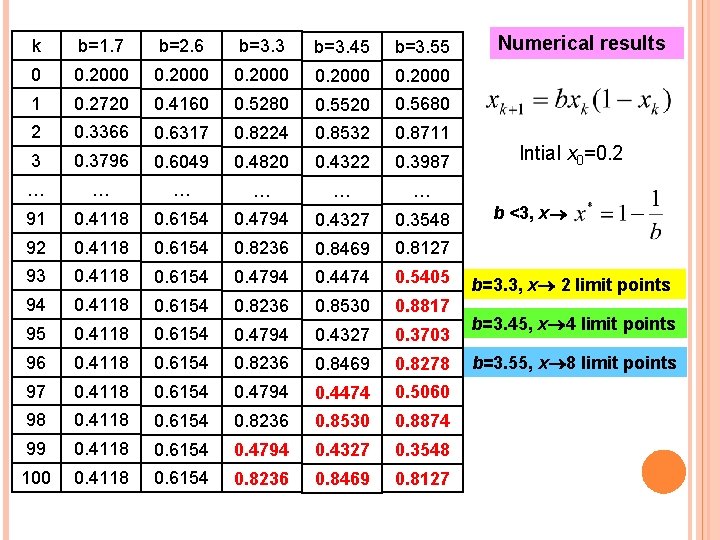
k b=1. 7 b=2. 6 b=3. 3 b=3. 45 b=3. 55 0 0. 2000 1 0. 2720 0. 4160 0. 5280 0. 5520 0. 5680 2 0. 3366 0. 6317 0. 8224 0. 8532 0. 8711 3 0. 3796 0. 6049 0. 4820 0. 4322 0. 3987 … … … 91 0. 4118 0. 6154 0. 4794 0. 4327 0. 3548 92 0. 4118 0. 6154 0. 8236 0. 8469 0. 8127 93 0. 4118 0. 6154 0. 4794 0. 4474 0. 5405 94 0. 4118 0. 6154 0. 8236 0. 8530 0. 8817 95 0. 4118 0. 6154 0. 4794 0. 4327 0. 3703 96 0. 4118 0. 6154 0. 8236 0. 8469 0. 8278 97 0. 4118 0. 6154 0. 4794 0. 4474 0. 5060 98 0. 4118 0. 6154 0. 8236 0. 8530 0. 8874 99 0. 4118 0. 6154 0. 4794 0. 4327 0. 3548 100 0. 4118 0. 6154 0. 8236 0. 8469 0. 8127 Numerical results Intial x 0=0. 2 b <3, x b=3. 3, x 2 limit points b=3. 45, x 4 limit points b=3. 55, x 8 limit points

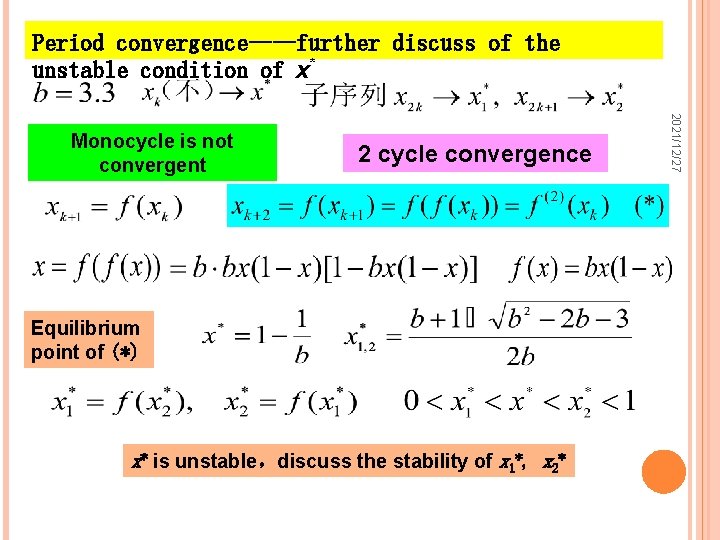
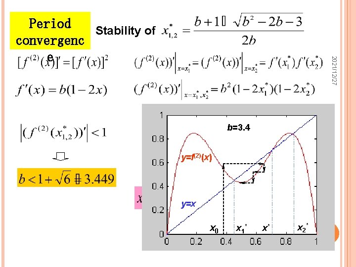
Period convergence——further discuss of the unstable condition of x* 2 cycle convergence Equilibrium point of (*) x* is unstable，discuss the stability of x 1*, x 2* 2021/12/27 Monocycle is not convergent

2021/12/27 Period Stability of convergenc e b=3. 4 y=f(2)(x) y=x x 0 x 1 * x* x 2 *

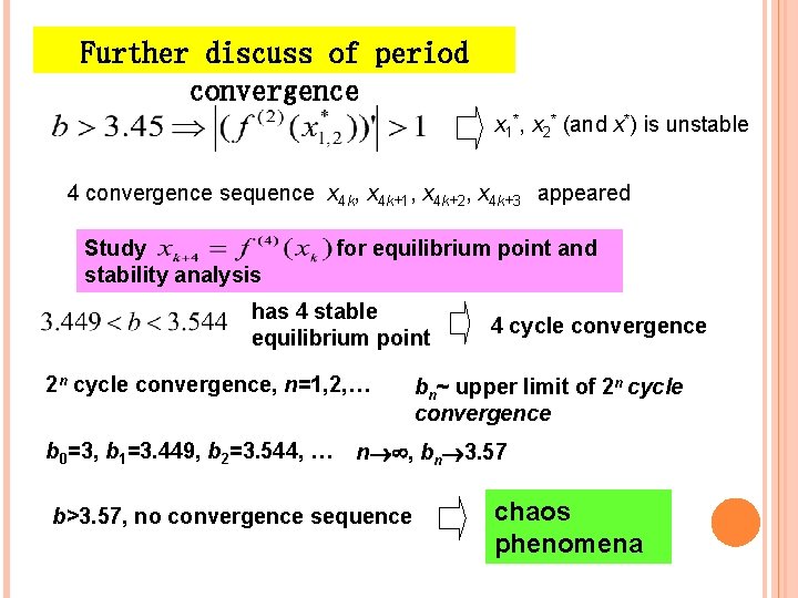
Further discuss of period convergence x 1*, x 2* (and x*) is unstable 4 convergence sequence x 4 k, x 4 k+1, x 4 k+2, x 4 k+3 appeared Study stability analysis for equilibrium point and has 4 stable equilibrium point 2 n cycle convergence, n=1, 2, … b 0=3, b 1=3. 449, b 2=3. 544, … 4 cycle convergence bn~ upper limit of 2 n cycle convergence n , bn 3. 57 b>3. 57, no convergence sequence chaos phenomena

2021/12/27 The End