MANE 4240 CIVL 4240 Introduction to Finite Elements

MANE 4240 & CIVL 4240 Introduction to Finite Elements Prof. Suvranu De Practical considerations in FEM modeling

Reading assignment: Logan Chap 7 + Lecture notes Summary: • Aspect ratio and element shapes • Use of symmetry • Natural subdivisions at discontinuities • Stress equilibrium in FEM solutions

© 2002 Brooks/Cole Publishing / Thomson Learning™ Aspect ratio and element shapes Aspect ratio = longest dimension/ shortest dimension Figure 7 -1 a (a) Beam with loading: effects of the aspect ratio (AR) illustrated by the five cases with different aspect ratios

© 2002 Brooks/Cole Publishing / Thomson Learning™ Figure 7 -1 b (b) Inaccuracy of solution as a function of the aspect ratio (numbers in parentheses correspond to the cases listed in Table 7 -1)

© 2002 Brooks/Cole Publishing / Thomson Learning™ Figure 7 -2 Elements with poor shapes

Avoid abrupt changes in element sizes Abrupt change in element size Gradual change in element size

Examples of how NOT to connect elements

Use of symmetry in modeling © 2002 Brooks/Cole Publishing / Thomson Learning™ Figure 7 -3 Use of symmetry applied to a soil mass subjected to foundation loading (number of nodes = 66, number of elements = 50) (2. 54 cm = 1 in. , 4. 445 N = 1 lb)

© 2002 Brooks/Cole Publishing / Thomson Learning™ Figure 7 -4 Use of symmetry applied to a uniaxially loaded member with a fillet

© 2002 Brooks/Cole Publishing / Thomson Learning™ Figure 7 -5 Problem reduction using axes of symmetry applied to a plate with a hole subjected to tensile force

Natural subdivisions at discontinuities

Look before you leap! 1. Check the model that you have developed: • Boundary conditions • Loadings • Symmetry? • Element aspect ratios/shapes • Mesh gradation 2. Check the results • Eyeball • Anything funny (nonzero displacements where they should be zero? ) • Are stress concentrations in places that you expect? • Comparison with known analytical solution/literature 3. If you remesh the same problem and analyze, do the solutions converge? (specifically check for convergence in strain energy)

Stress equilibrium in FEM analysis Example: Consider a linear elastic bar with varying cross section 2 1 x 80 cm P=3 E/80 E: Young’s modulus Boundary conditions Analytical solution The governing differential (equilibrium) equation Eq(1)

Lets us discretize the bar using a 2 -noded (linear) bar element. The finite element approximation within the bar is where the shape functions If we incorporate the boundary condition at x=0 Does this solution satisfy the equilibrium equation (Eq 1)?

Conclusion: The FEM displacement field does NOT satisfy the equilibrium equations at every point inside the elements. However, the solution gets better as the mesh is refined.

Stress equilibrium in FEM analysis To obtain exact solution of the mathematical model in solid mechanics we need to satisfy 1. Compatibility 2. Stress-strain law 3. Stress-equilibrium at every point in the computational domain. In a FE model one satisfies the first 2 conditions exactly. But stress-equilibrium is NOT satisfied point wise. Question: Then what is satisfied?

Let us compute the FEM solution using a bar element The stiffness matrix is The system equations to solve are With u 1 x=0; we solve for (Note that the exact solution for the displacement at node 2 is 1 cm!!)

Let us now compute the nodal forces due to element stresses using the formula

Two observations P=3 E/80 1. Element equilibrium 2. Nodal equilibrium

The following two properties are ALWAYS satisfied by the FEM solution using a coarse or a fine mesh P Property 1: Nodal point equilibrium Property 2. Element equilibrium El #4 El #2 El #3 El #1 PROPERTY 1: (Nodal point equilibrium) At any node the sum of the element nodal point forces is in equilibrium with the externally applied loads (including all effects due to body forces, surface tractions, initial stresses, concentrated loads, inertia, damping and reaction)

How to compute the nodal reaction forces for a given finite element? Once we have computed the element stress, we may obtain the nodal reaction forces as

Nodal point equilibrium implies: P El #4 El #2 El #3 El #1 Sum of forces equal externally applied load (=0 at this node) This is equal in magnitude and in the same direction as P

PROPERTY 2: (Element equilibrium) Each element is in equilibrium under its forces f i. e. , each element is under force and moment equilibrium e. g. , Define F 4 y as a rigid body displacement in x-direction F 3 y F 3 x F 4 x But F 2 x F 1 y Hence F 2 y since this is a rigid body displacement, the strains are zero

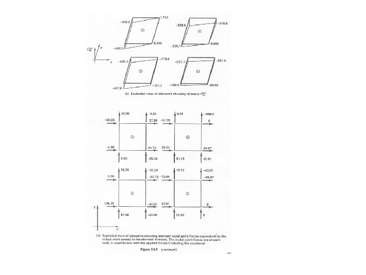
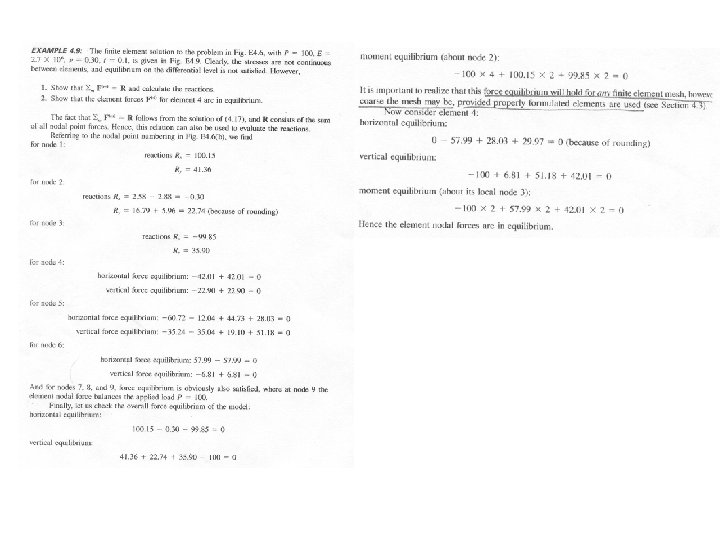
Example (Finite Element Procedures, Bathe 1996)

NOTE: In a finite element analysis 1. Stress equilibrium violated inside each element 2. Stresses are discontinuous across elements 3. Stresses are not in equilibrium with the applied traction

© 2002 Brooks/Cole Publishing / Thomson Learning™ Figure 7 -10 Example 6. 2, illustrating violation of equilibrium of a differential element and along the diagonal edge between two elements (the coarseness of the mesh amplifies the violation of equilibrium)

© 2002 Brooks/Cole Publishing / Thomson Learning™ Figure 7 -11 Convergence of a finite element solution based on the compatible displacement formulation

Hence a finite element analysis can be interpreted as a process in which 1. The structure or continuum is idealized as an assemblage of elements connected at nodes pertaining to the elements. 2. The externally applied forces are lumped to these nodes to obtain the equivalent nodal load vectors 3. The equivalent nodal loads are equilibriated by the nodal point forces that are equivalent to the element internal stresses. 4. Compatibility and stress-strain relationships are exactly satisfied, but instead of force equilibrium at the differential level, only global equilibrium for the complete structure, of the nodal points and of each element under its nodal point forces is satisfied.