MANE 4240 CIVL 4240 Introduction to Finite Elements

MANE 4240 & CIVL 4240 Introduction to Finite Elements Prof. Suvranu De Development of Truss Equations

Reading assignment: Chapter 3: Sections 3. 1 -3. 9 + Lecture notes Summary: • Stiffness matrix of a bar/truss element • Coordinate transformation • Stiffness matrix of a truss element in 2 D space • Problems in 2 D truss analysis (including multipoint constraints) • 3 D Truss element

Trusses: Engineering structures that are composed only of two-force members. e. g. , bridges, roof supports Actual trusses: Airy structures composed of slender members (I-beams, channels, angles, bars etc) joined together at their ends by welding, riveted connections or large bolts and pins A typical truss structure Gusset plate

Ideal trusses: Assumptions • Ideal truss members are connected only at their ends. • Ideal truss members are connected by frictionless pins (no moments) • The truss structure is loaded only at the pins • Weights of the members are neglected A typical truss structure Frictionless pin

These assumptions allow us to idealize each truss member as a two-force member (members loaded only at their extremities by equal opposite and collinear forces) member in compression member in tension Connecting pin

FEM analysis scheme Step 1: Divide the truss into bar/truss elements connected to each other through special points (“nodes”) Step 2: Describe the behavior of each bar element (i. e. derive its stiffness matrix and load vector in local AND global coordinate system) Step 3: Describe the behavior of the entire truss by putting together the behavior of each of the bar elements (by assembling their stiffness matrices and load vectors) Step 4: Apply appropriate boundary conditions and solve

Stiffness matrix of bar element E, A © 2002 Brooks/Cole Publishing / Thomson Learning™ L: Length of bar A: Cross sectional area of bar E: Elastic (Young’s) modulus of bar : displacement of bar as a function of local coordinate The strain in the bar at The stress in the bar (Hooke’s law) of bar

Tension in the bar Assume that the displacement L is varying linearly along the bar Then, strain is constant along the bar: Stress is also constant along the bar: Tension is constant along the bar: The bar is acting like a spring with stiffness

Recall the lecture on springs E, A © 2002 Brooks/Cole Publishing / Thomson Learning™ Two nodes: 1, 2 Nodal displacements: Nodal forces: Spring constant: Element stiffness matrix in local coordinates Element force vector Element stiffness matrix Element nodal displacement vector

What if we have 2 bars? E 1, A 1 E 2, A 2 L 1 This is equivalent to the following system of springs x Element 1 2 Element 23 1 d 1 x PROBLEM d 2 x d 3 x

Problem 1: Find the stresses in the two-bar assembly loaded as shown below E, 2 A E, A P 1 2 3 L L Solution: This is equivalent to the following system of springs x Element 1 2 Element 23 1 d 1 x d 2 x d 3 x We will first compute the displacement at node 2 and then the stresses within each element

The global set of equations can be generated using the technique developed in the lecture on “springs” here Hence, the above set of equations may be explicitly written as From equation (2)

To calculate the stresses: For element #1 first compute the element strain and then the stress as (element in tension) Similarly, in element # 2 (element in compression)

© 2002 Brooks/Cole Publishing / Thomson Learning™ Inter-element continuity of a two-bar structure

Bars in a truss have various orientations member in compression member in tension Connecting pin

y x At node 1: At node 2:

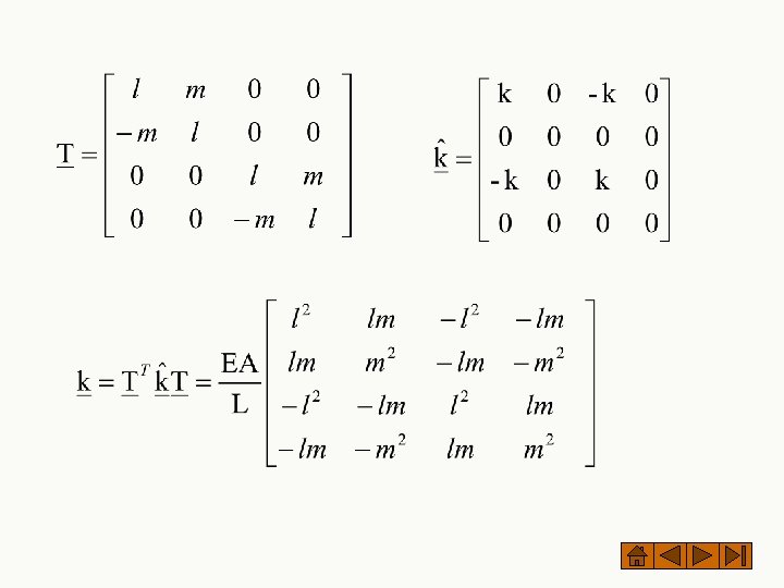
In the global coordinate system, the vector of nodal displacements and loads Our objective is to obtain a relation of the form Where k is the 4 x 4 element stiffness matrix in global coordinate system

The key is to look at the local coordinates y x Rewrite as

NOTES 1. Assume that there is no stiffness in the local ^y direction. 2. If you consider the displacement at a point along the local x direction as a vector, then the components of that vector along the global x and y directions are the global x and y displacements. 3. The expanded stiffness matrix in the local coordinates is symmetric and singular.

NOTES 5. In local coordinates we have But or goal is to obtain the following relationship Hence, need a relationship between and and Need to understand how the components of a vector change with coordinate transformation

Transformation of a vector in two dimensions y v Angle q is measured positive in the counter clockwise direction from the +x axis) x The vector v has components (vx, vy) in the global coordinate system and (v^x, v^y) in the local coordinate system. From geometry

In matrix form Direction cosines Or where Transformation matrix for a single vector in 2 D relates where are components of the same vector in local and global coordinates, respectively.

Relationship between At node 1 At node 2 Putting these together and for the truss element

Relationship between At node 1 At node 2 Putting these together and for the truss element

Important property of the transformation matrix T The transformation matrix is orthogonal, i. e. its inverse is its transpose Use the property that l 2+m 2=1

Putting all the pieces together y x The desired relationship is Where is the element stiffness matrix in the global coordinate system

Computation of the direction cosines L 1 2 (x 2, y 2) (x 1, y 1) What happens if I reverse the node numbers? L 2 (x , y ) 2 2 Question: Does the stiffness matrix change? 1 (x 1, y 1)

Example Bar element for stiffness matrix evaluation © 2002 Brooks/Cole Publishing / Thomson Learning™

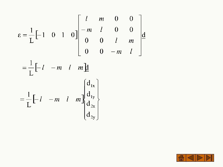
Computation of element strains © 2002 Brooks/Cole Publishing / Thomson Learning™ Recall that the element strain is

Computation of element stresses stress and tension Recall that the element stress is Recall that the element tension is

Steps in solving a problem Step 1: Write down the node-element connectivity table linking local and global nodes; also form the table of direction cosines (l, m) Step 2: Write down the stiffness matrix of each element in global coordinate system with global numbering Step 3: Assemble the element stiffness matrices to form the global stiffness matrix for the entire structure using the node element connectivity table Step 4: Incorporate appropriate boundary conditions Step 5: Solve resulting set of reduced equations for the unknown displacements Step 6: Compute the unknown nodal forces

Node element connectivity table ELEMENT Node 1 Node 2 1 1 2 2 2 3 3 3 1 1 El 1 2 60 60 L El 3 60 El 2 3 1 (x 1, y 1) 2 (x 2, y 2)

Stiffness matrix of element 1 d 1 x d 1 y d 2 x d 2 y d 1 x Stiffness matrix of element 2 d 2 x d 2 y d 3 x d 3 y d 2 x d 1 y d 2 x d 3 x d 2 y d 3 y Stiffness matrix of element 3 d 3 x d 3 y d 1 x d 1 y There are 4 degrees of freedom (dof) per element (2 per node)

Global stiffness matrix d 1 y d 2 x d 2 y d 3 x d 3 y d 1 x d 1 y d 2 x d 2 y d 3 x d 3 y How do you incorporate boundary conditions?

Example 2 y 3 The length of bars 12 and 23 are equal (L) E: Young’s modulus A: Cross sectional area of each bar Solve for P 1 (1) d and d 2 x 2 y (2) Stresses in each bar El#2 P 2 El#1 2 45 o 1 x Solution Step 1: Node element connectivity table ELEMENT Node 1 Node 2 1 1 2 2 2 3

Table of nodal coordinates Node x y 1 0 0 2 Lcos 45 Lsin 45 3 0 2 Lsin 45 Table of direction cosines ELEMENT Length 1 L cos 45 sin 45 2 L -cos 45 sin 45

Step 2: Stiffness matrix of each element in global coordinates with global numbering Stiffness matrix of element 1 d 1 x d 1 y d 2 x d 2 y

Stiffness matrix of element 2 d 2 x d 2 y d 3 x d 3 y

Step 3: Assemble the global stiffness matrix The final set of equations is

Step 4: Incorporate boundary conditions Hence reduced set of equations to solve for unknown displacements at node 2

Step 5: Solve for unknown displacements Step 6: Obtain stresses in the elements 0 For element #1: 0

For element #2: 0 0

Multi-point constraints © 2002 Brooks/Cole Publishing / Thomson Learning™ Figure 3 -19 Plane truss with inclined boundary conditions at node 3 (see problem worked out in class)

Problem 3: For the plane truss y P 3 El#2 2 El#1 El#3 45 o 1 x P=1000 k. N, L=length of elements 1 and 2 = 1 m E=210 GPa A = 6× 10 -4 m 2 for elements 1 and 2 = 6 × 10 -4 m 2 for element 3 Determine the unknown displacements and reaction forces. Solution Step 1: Node element connectivity table ELEMENT Node 1 Node 2 1 1 2 2 2 3 3 1 3

Table of nodal coordinates Node x y 1 0 0 2 0 L 3 L L Table of direction cosines ELEMENT Length 1 L 0 1 2 L 1 0 3 L

Step 2: Stiffness matrix of each element in global coordinates with global numbering Stiffness matrix of element 1 d 1 x d 1 y d 2 x d 2 y

Stiffness matrix of element 2 d 2 x d 2 y d 3 x d 3 y Stiffness matrix of element 3 d 1 x d 1 y d 3 x d 3 y

Step 3: Assemble the global stiffness matrix N/m The final set of equations is Eq(1)

Step 4: Incorporate boundary conditions y P 3 El#2 2 El#1 El#3 45 o 1 Also, x in the local coordinate system of element 3 How do I convert this to a boundary condition in the global (x, y) coordinates?

y P 3 El#2 2 El#1 El#3 45 o 1 Also, x in the local coordinate system of element 3 How do I convert this to a boundary condition in the global (x, y) coordinates?

Using coordinate transformations (Multi-point constraint) Eq (2)

Similarly for the forces at node 3 Eq (3)

Therefore we need to solve the following equations simultaneously Eq(1) Eq(2) Eq(3) Incorporate boundary conditions and reduce Eq(1) to

Write these equations out explicitly Eq(4) Eq(5) Eq(6) Add Eq (5) and (6) using Eq(3) using Eq(2) Eq(7) Plug this into Eq(4)

Compute the reaction forces

Physical significance of the stiffness matrix In general, we will have a stiffness matrix of the form And the finite element force-displacement relation

Physical significance of the stiffness matrix The first equation is Force equilibrium equation at node 1 Columns of the global stiffness matrix What if d 1=1, d 2=0, d 3=0 ? While d. o. f 2 and 3 are held fixed Force along d. o. f 1 due to unit displacement at d. o. f 1 Force along d. o. f 2 due to unit displacement at d. o. f 1 Force along d. o. f 3 due to unit displacement at d. o. f 1 Similarly we obtain the physical significance of the other entries of the global stiffness matrix

In general = Force at d. o. f ‘i’ due to unit displacement at d. o. f ‘j’ keeping all the other d. o. fs fixed

Example y 3 The length of bars 12 and 23 are equal (L) E: Young’s modulus A: Cross sectional area of each bar Solve for d 2 x and d 2 y using the “physical P 1 interpretation” approach El#2 P 2 El#1 2 45 o 1 x Solution Notice that the final set of equations will be of the form Where k 11, k 12, k 21 and k 22 will be determined using the “physical interpretation” approach

To obtain the first column y 3 El#1 1 y F 2 y=k 21 El#2 F 2 x=k 11 2’ 2 x apply T 2 T 1 F 2 y=k 21 F 2 x=k 11 2 x d 2 x=1 Force equilibrium Force-deformation relations

Combining force equilibrium and force-deformation relations Now use the geometric (compatibility) conditions (see figure) Finally

To obtain the second column y y 3 El#2 El#1 1 apply 2’ 2 d 2 y=1 T 2 T 1 x Force equilibrium F 2 y=k 22 F 2 x=k 12 2 x Force-deformation relations

Combining force equilibrium and force-deformation relations Now use the geometric (compatibility) conditions (see figure) This negative is due to compression Finally

© 2002 Brooks/Cole Publishing / Thomson Learning™ 3 D Truss (space truss)

In local coordinate system

The transformation matrix for a single vector in 3 D l 1, m 1 and n 1 are the direction cosines of x^ © 2002 Brooks/Cole Publishing / Thomson Learning™

Transformation matrix T relating the local and global displacement and load vectors of the truss element Element stiffness matrix in global coordinates

Notice that the direction cosines of only the local ^x axis enter the k matrix