Investment Analysis and Portfolio Management Lecture 3 Gareth

Investment Analysis and Portfolio Management Lecture 3 Gareth Myles

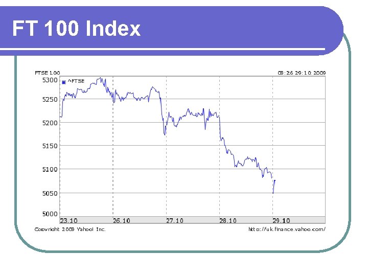
FT 100 Index

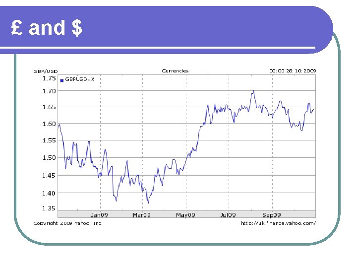
£ and $

Risk l Variance The standard measure of risk is the variance of return or l Its square root: the standard deviation l l Sample l variance The value obtained from past data l Population l variance The value from the true model of the data

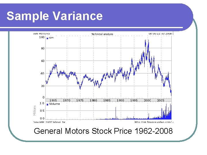
Sample Variance General Motors Stock Price 1962 -2008

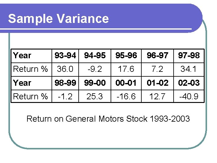
Sample Variance Year Return % 93 -94 94 -95 36. 0 -9. 2 98 -99 99 -00 -1. 2 25. 3 95 -96 96 -97 97 -98 17. 6 7. 2 34. 1 00 -01 01 -02 02 -03 -16. 6 12. 7 -40. 9 Return on General Motors Stock 1993 -2003

Sample Variance Graph of return

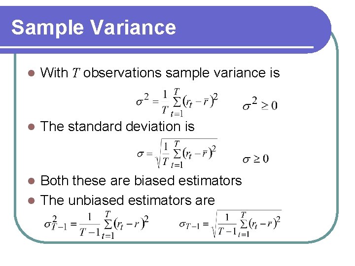
Sample Variance l With T observations sample variance is l The standard deviation is Both these are biased estimators l The unbiased estimators are l

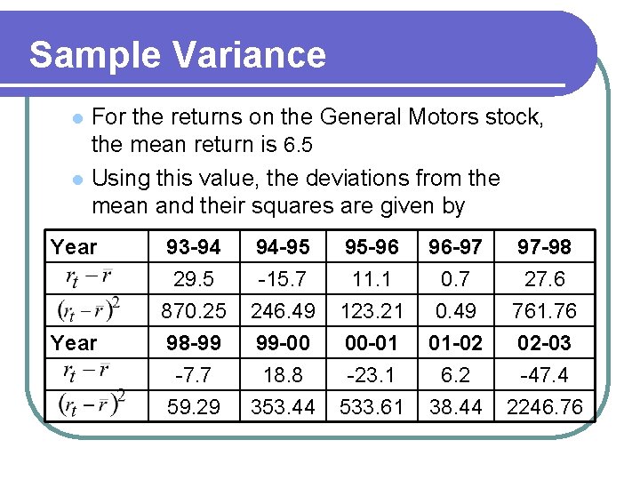
Sample Variance l l For the returns on the General Motors stock, the mean return is 6. 5 Using this value, the deviations from the mean and their squares are given by Year 93 -94 29. 5 870. 25 98 -99 94 -95 -15. 7 246. 49 99 -00 95 -96 11. 1 123. 21 00 -01 96 -97 0. 49 01 -02 97 -98 27. 6 761. 76 02 -03 -7. 7 59. 29 18. 8 353. 44 -23. 1 533. 61 6. 2 38. 44 -47. 4 2246. 76

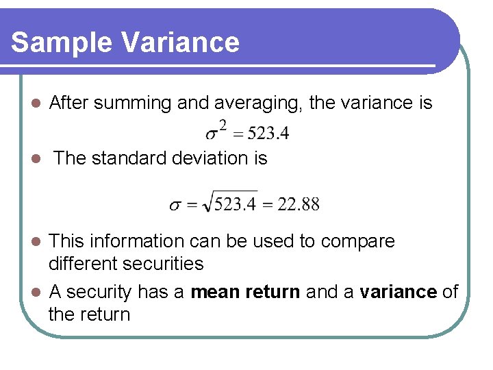
Sample Variance l l After summing and averaging, the variance is The standard deviation is This information can be used to compare different securities l A security has a mean return and a variance of the return l

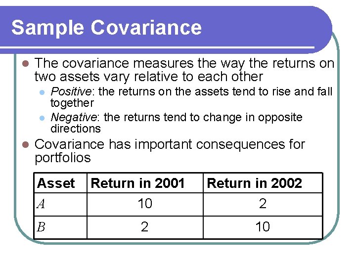
Sample Covariance l The covariance measures the way the returns on two assets vary relative to each other l l l Positive: the returns on the assets tend to rise and fall together Negative: the returns tend to change in opposite directions Covariance has important consequences for portfolios Asset A B Return in 2001 10 2 Return in 2002 2 10

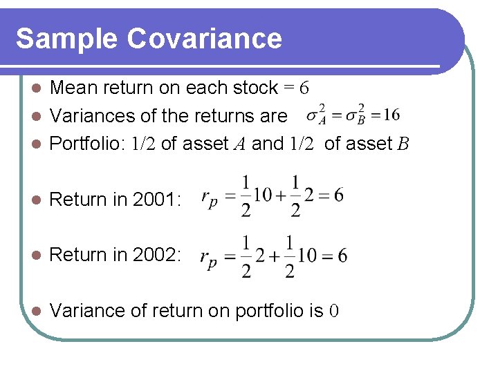
Sample Covariance Mean return on each stock = 6 l Variances of the returns are l Portfolio: 1/2 of asset A and 1/2 of asset B l l Return in 2001: l Return in 2002: l Variance of return on portfolio is 0

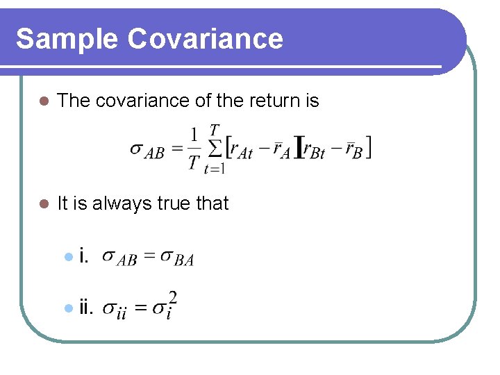
Sample Covariance l The covariance of the return is l It is always true that l ii.

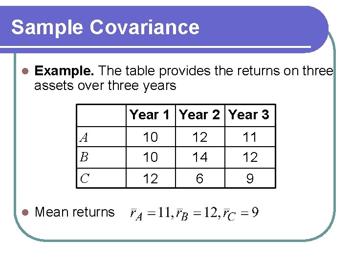
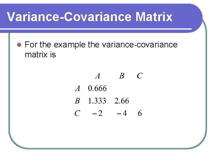
Sample Covariance l Example. The table provides the returns on three assets over three years Year 1 Year 2 Year 3 l A B 10 10 12 14 11 12 C 12 6 9 Mean returns

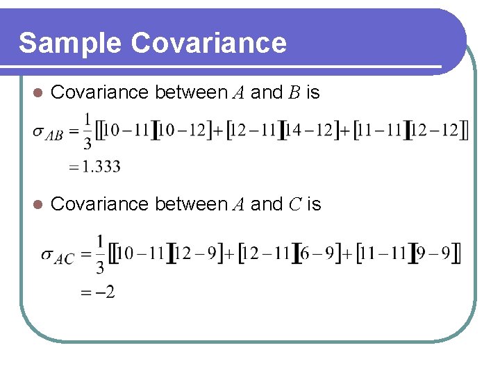
Sample Covariance l Covariance between A and B is l Covariance between A and C is

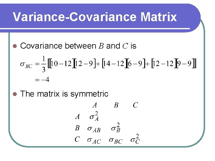
Variance-Covariance Matrix l Covariance between B and C is l The matrix is symmetric

Variance-Covariance Matrix l For the example the variance-covariance matrix is

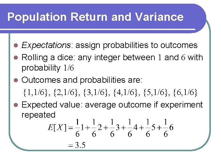
Population Return and Variance Expectations: assign probabilities to outcomes l Rolling a dice: any integer between 1 and 6 with probability 1/6 l Outcomes and probabilities are: {1, 1/6}, {2, 1/6}, {3, 1/6}, {4, 1/6}, {5, 1/6}, {6, 1/6} l Expected value: average outcome if experiment repeated l

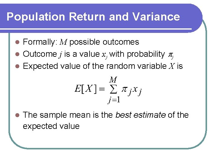
Population Return and Variance Formally: M possible outcomes l Outcome j is a value xj with probability pj l Expected value of the random variable X is l l The sample mean is the best estimate of the expected value

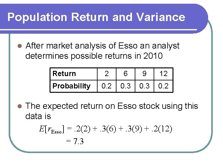
Population Return and Variance l After market analysis of Esso an analyst determines possible returns in 2010 Return Probability l 2 6 9 12 0. 3 0. 2 The expected return on Esso stock using this data is E[r. Esso] =. 2(2) +. 3(6) +. 3(9) +. 2(12) = 7. 3

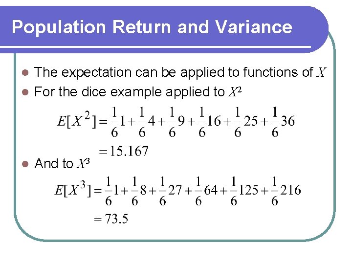
Population Return and Variance The expectation can be applied to functions of X l For the dice example applied to X 2 l l And to X 3

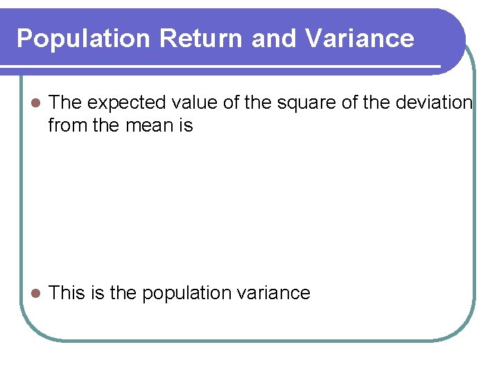
Population Return and Variance l The expected value of the square of the deviation from the mean is l This is the population variance

Modelling Returns l States of the world l l Provide a summary of the information about future return on an asset A way of modelling the randomness in asset returns l Not intended as a practical description

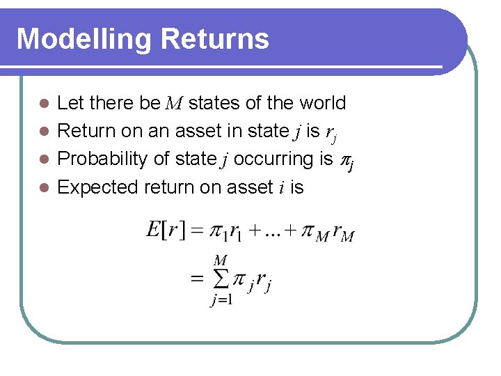
Modelling Returns Let there be M states of the world l Return on an asset in state j is rj l Probability of state j occurring is pj l Expected return on asset i is l

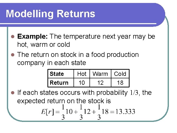
Modelling Returns Example: The temperature next year may be hot, warm or cold l The return on stock in a food production company in each state l State Return l Hot 10 Warm Cold 12 18 If each states occurs with probability 1/3, the expected return on the stock is

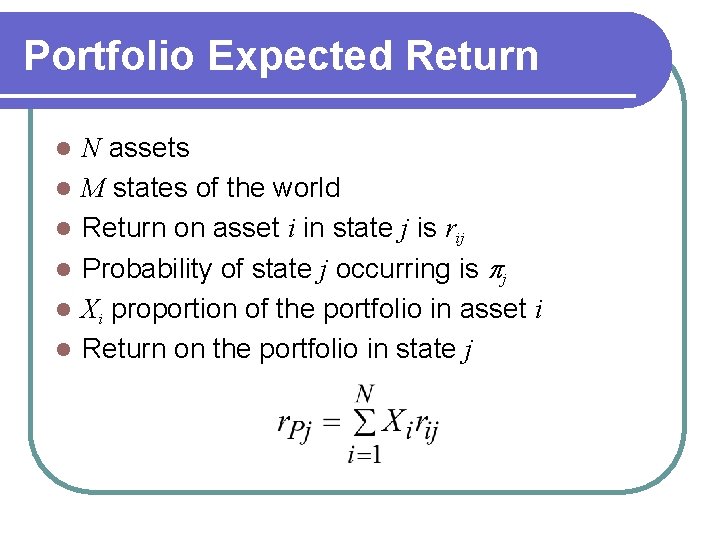
Portfolio Expected Return l l l N assets M states of the world Return on asset i in state j is rij Probability of state j occurring is pj Xi proportion of the portfolio in asset i Return on the portfolio in state j

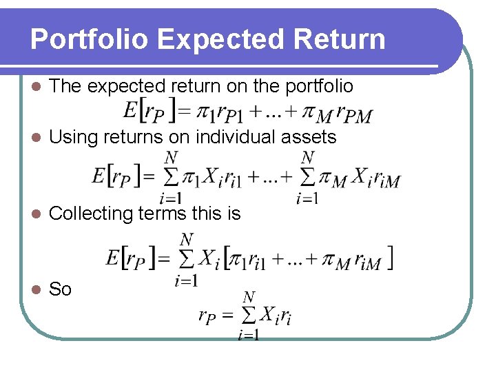
Portfolio Expected Return l The expected return on the portfolio l Using returns on individual assets l Collecting terms this is l So

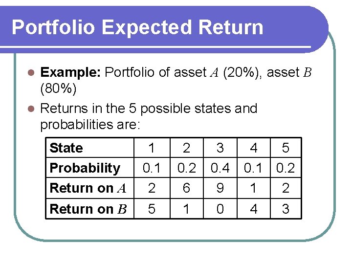
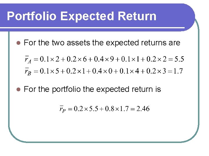
Portfolio Expected Return Example: Portfolio of asset A (20%), asset B (80%) l Returns in the 5 possible states and probabilities are: l State Probability Return on A 1 0. 1 2 2 0. 2 6 3 0. 4 9 Return on B 5 1 0 4 5 0. 1 0. 2 1 2 4 3

Portfolio Expected Return l For the two assets the expected returns are l For the portfolio the expected return is

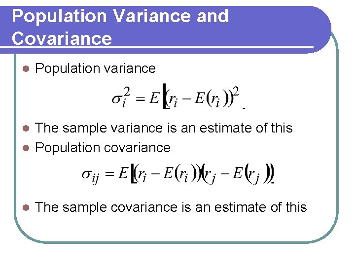
Population Variance and Covariance l Population variance The sample variance is an estimate of this l Population covariance l l The sample covariance is an estimate of this

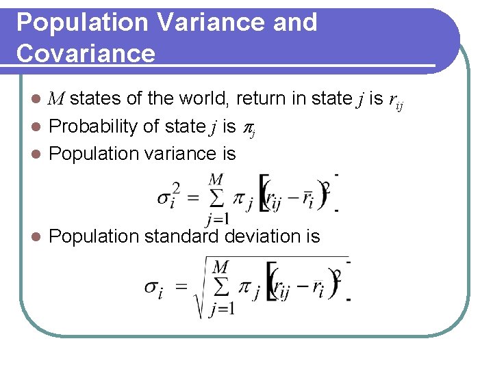
Population Variance and Covariance M states of the world, return in state j is rij l Probability of state j is pj l Population variance is l l Population standard deviation is

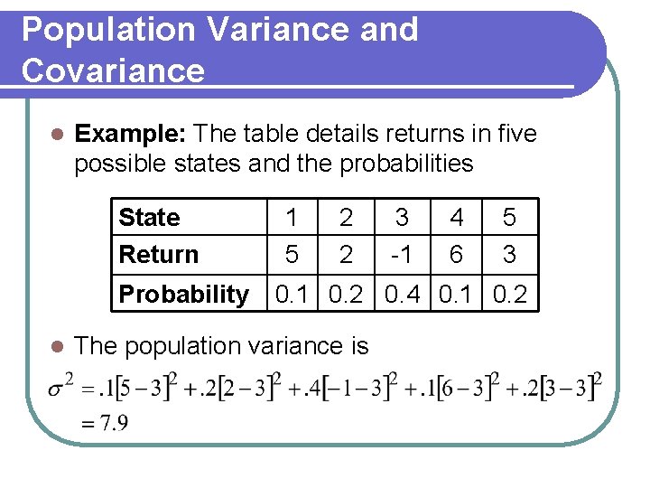
Population Variance and Covariance l Example: The table details returns in five possible states and the probabilities State Return Probability l 1 5 2 2 3 -1 4 6 5 3 0. 1 0. 2 0. 4 0. 1 0. 2 The population variance is

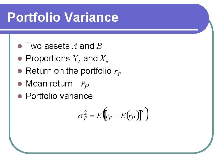
Portfolio Variance l l l Two assets A and B Proportions XA and XB Return on the portfolio r. P Mean return Portfolio variance

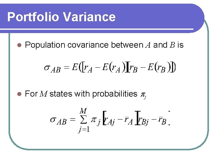
Portfolio Variance l Population covariance between A and B is l For M states with probabilities pj

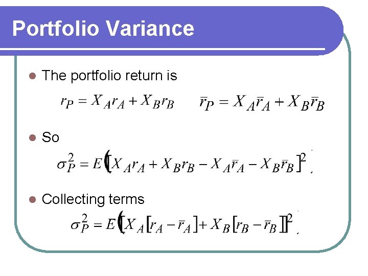
Portfolio Variance l The portfolio return is l So l Collecting terms

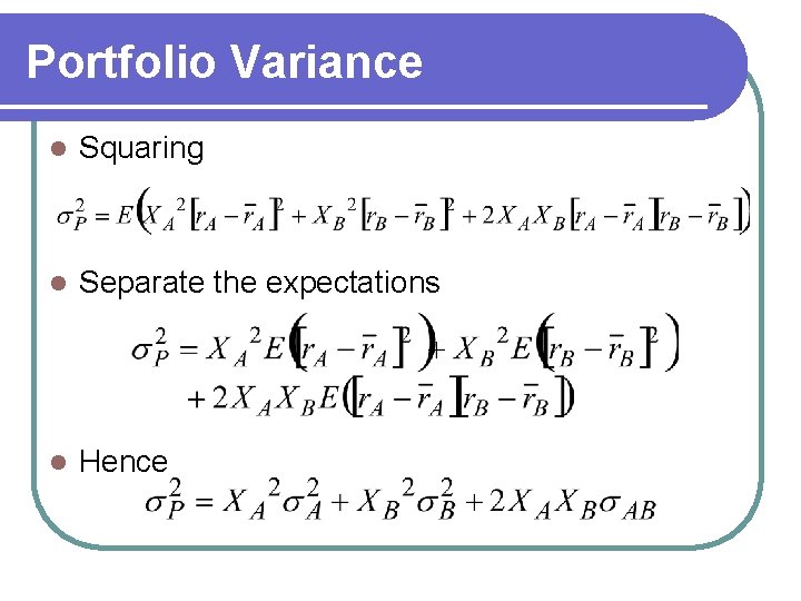
Portfolio Variance l Squaring l Separate the expectations l Hence

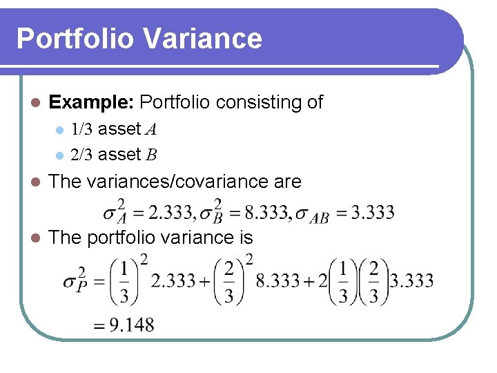
Portfolio Variance l Example: Portfolio consisting of l l 1/3 asset A 2/3 asset B l The variances/covariance are l The portfolio variance is

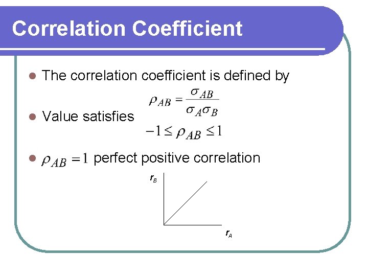
Correlation Coefficient l The correlation coefficient is defined by l Value satisfies l perfect positive correlation r. B r. A

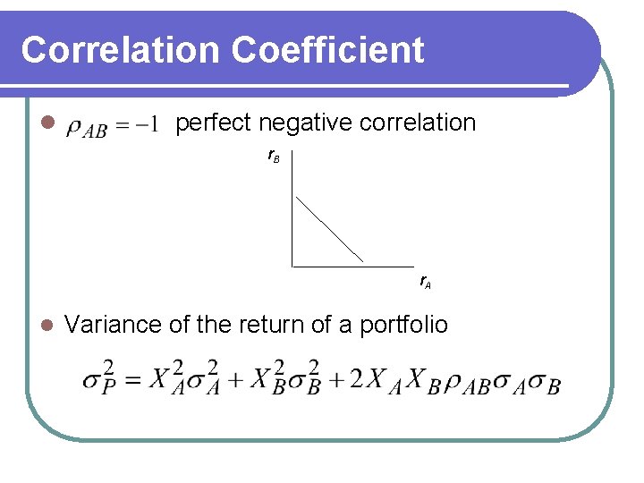
Correlation Coefficient l perfect negative correlation r. B r. A l Variance of the return of a portfolio

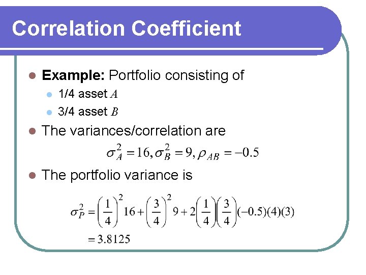
Correlation Coefficient l Example: Portfolio consisting of l l 1/4 asset A 3/4 asset B l The variances/correlation are l The portfolio variance is

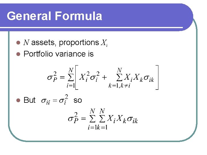
General Formula N assets, proportions Xi l Portfolio variance is l l But so

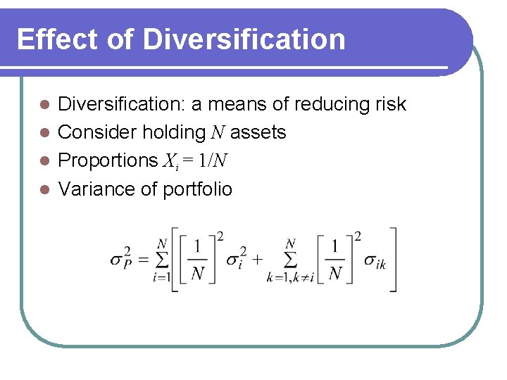
Effect of Diversification: a means of reducing risk l Consider holding N assets l Proportions Xi = 1/N l Variance of portfolio l

Effect of Diversification N terms in the first summation, N[ N-1] in the second l Gives l l Define l Then

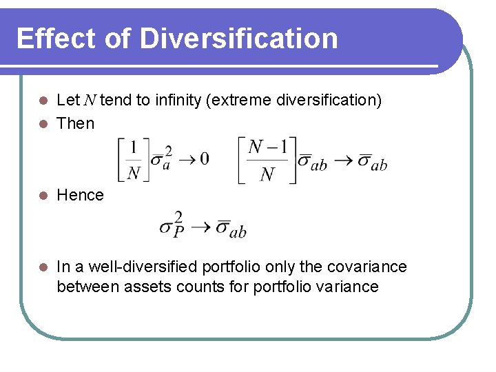
Effect of Diversification Let N tend to infinity (extreme diversification) l Then l l Hence l In a well-diversified portfolio only the covariance between assets counts for portfolio variance