Investment Analysis and Portfolio Management Lecture 7 Gareth

Investment Analysis and Portfolio Management Lecture 7 Gareth Myles

The Capital Asset Pricing Model (CAPM) l The CAPM is a model of equilibrium in the market for securities. l Previous lectures have addressed the question of how investors should choose assets given the observed structure of returns. l Now the question is changed to: l If investors follow these strategies, how will returns be determined in equilibrium?

The Capital Asset Pricing Model (CAPM) l The simplest and most fundamental model of equilibrium in the security market l l Builds on the Markowitz model of portfolio choice Aggregates the choices of individual investors Trading ensures an equilibrium where returns adjust so that the demand supply of assets are equal l Many modifications/extensions can be made l l But basic insights always extend

Assumptions The CAPM is built on a set of assumptions l Individual investors l l l Investors evaluate portfolios by the mean and variance of returns over a one period horizon Preferences satisfy non-satiation Investors are risk averse Trading conditions l l l Assets are infinitely divisible Borrowing and lending can be undertaken at the risk-free rate of return There are no taxes or transactions costs

Assumptions The risk-free rate is the same for all l Information flows perfectly l l The set of investors All investors have the same time horizon l Investors have identical expectations l

Assumptions The first six assumptions are the Markowitz model l The seventh and eighth assumptions add a perfect capital market and perfect information l The final two assumptions make all investors identical except for their degree of risk aversion l

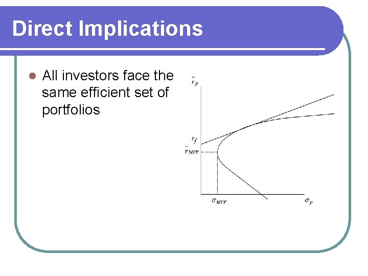
Direct Implications l All investors face the same efficient set of portfolios

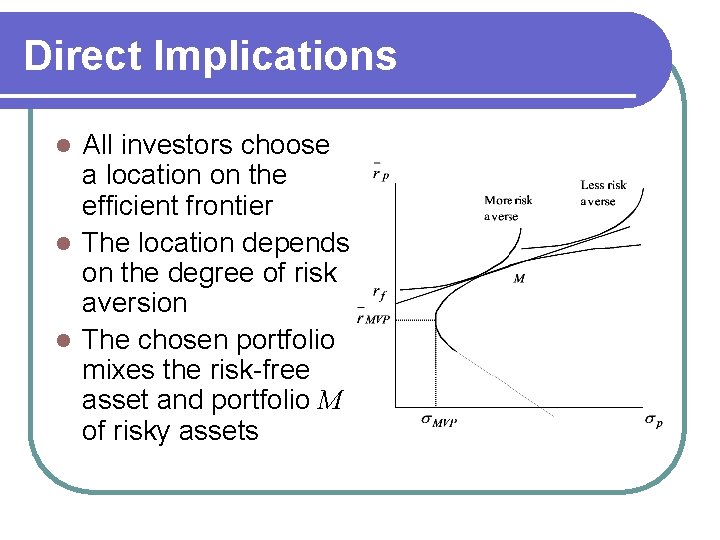
Direct Implications All investors choose a location on the efficient frontier l The location depends on the degree of risk aversion l The chosen portfolio mixes the risk-free asset and portfolio M of risky assets l

Separation Theorem l The optimal combination of risky assets is determined without knowledge of preferences l l l All choose portfolio M This is the Separation Theorem M must be the market portfolio of risky assets l l l All investors hold it to a greater or lesser extent No other portfolio of risky assets is held There is a question about the interpretation of this portfolio

Equilibrium l The only assets that need to be marketed are: l l The risk-free asset A mutual fund representing the market portfolio No other assets are required In equilibrium there can be no short sales of the risky assets l l l All investors buy the same risky assets No-one can be short since all would be short If all are short the market is not in equilibrium

Equilibrium l Equilibrium occurs when the demand for assets matches the supply l l This also applies to the risk-free Borrowing must equal lending This is achieved by the adjustment of asset prices l As prices change so do the returns on the assets l This process generates an equilibrium structure of returns l

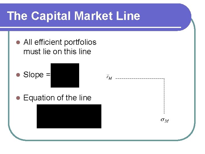
The Capital Market Line l All efficient portfolios must lie on this line l Slope = l Equation of the line

Interpretation l rf is the reward for "time" Patience is rewarded l Investment delays consumption l is the reward for accepting "risk" l The market price of risk l Judged to be equilibrium reward l Obtained by matching demand to supply l

Security Market Line l Now consider the implications for individual assets l Graph covariance against return The risk on the market portfolio is l The covariance of the risk-free asset is zero l The covariance of the market with the market is l

Security Market Line l Can mix M and the riskfree asset along the line l l l If there was a portfolio above the line all investors would buy it No investor would hold one below The equation of the line is M

Security Market Line l Define l The equation of the line becomes l This is the security market line (SML)

Security Market Line There is a linear trade-off between risk measured by and return l In equilibrium all assets and portfolios must have risk-return combinations that lie on this line l

Market Model and CAPM l Market model uses l CAPM uses l is derived from an assumption about the determination of returns it is derived from a statistical model l the index is chosen not specified by any underlying analysis l l is derived from an equilibrium theory

Market Model and CAPM l In addition: I is usually assumed to be the market index, but in principal could be any index l M is always the market portfolio l l There is a difference between these l But they are often used interchangeably l The market index is taken as an approximation of the market portfolio

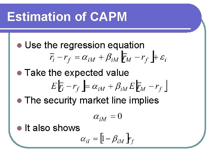
Estimation of CAPM l Use the regression equation l Take l The l It the expected value security market line implies also shows

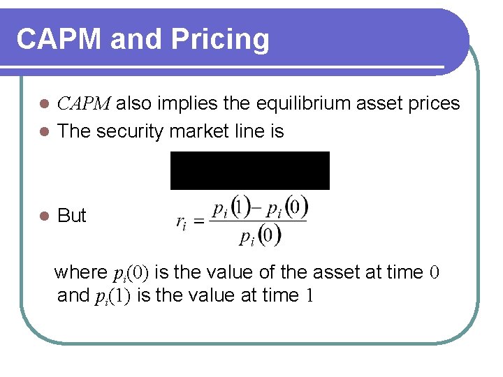
CAPM and Pricing CAPM also implies the equilibrium asset prices l The security market line is l l But where pi(0) is the value of the asset at time 0 and pi(1) is the value at time 1

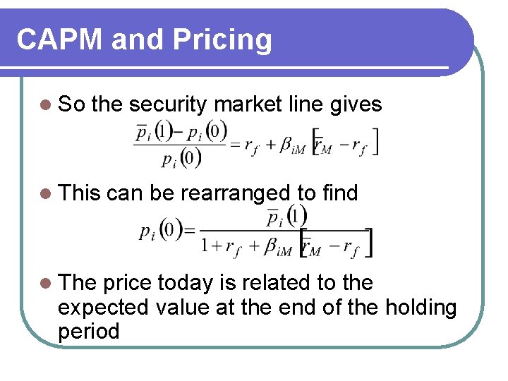
CAPM and Pricing l So the security market line gives l This l The can be rearranged to find price today is related to the expected value at the end of the holding period

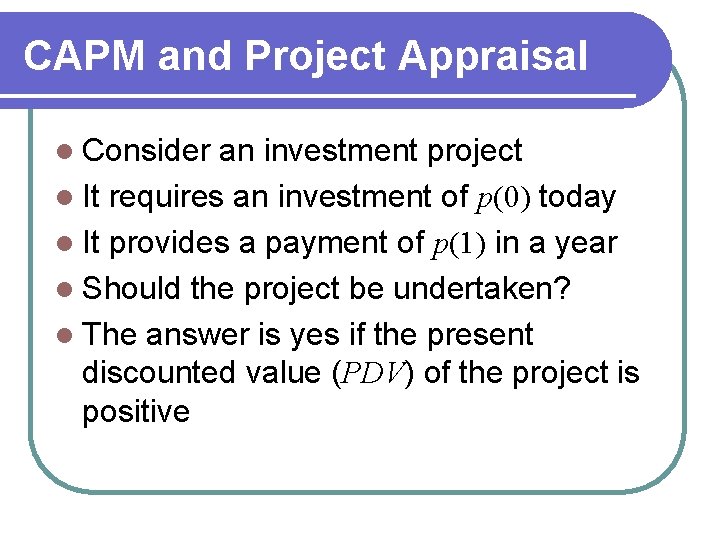
CAPM and Project Appraisal l Consider an investment project l It requires an investment of p(0) today l It provides a payment of p(1) in a year l Should the project be undertaken? l The answer is yes if the present discounted value (PDV) of the project is positive

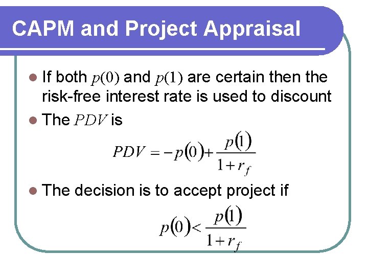
CAPM and Project Appraisal l If both p(0) and p(1) are certain the risk-free interest rate is used to discount l The PDV is l The decision is to accept project if

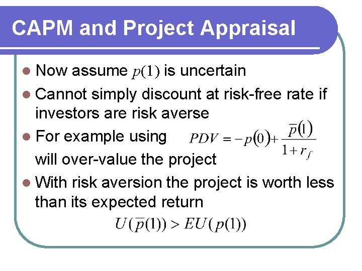
CAPM and Project Appraisal l Now assume p(1) is uncertain l Cannot simply discount at risk-free rate if investors are risk averse l For example using will over-value the project l With risk aversion the project is worth less than its expected return

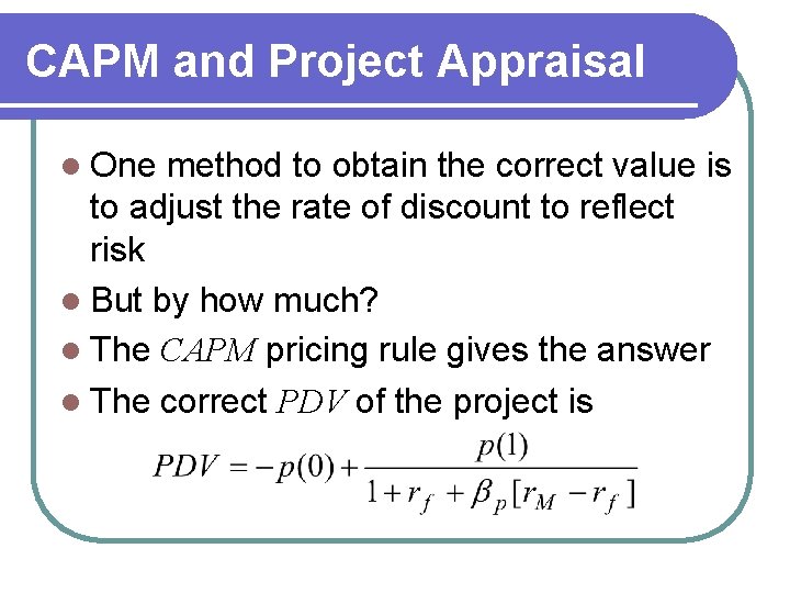
CAPM and Project Appraisal l One method to obtain the correct value is to adjust the rate of discount to reflect risk l But by how much? l The CAPM pricing rule gives the answer l The correct PDV of the project is