Introduction to Digital Image Processing DIP Weihua Zhou

Introduction to Digital Image Processing (DIP) Weihua Zhou

Outline z Digital Image and Digital Image Processing: examples z DIP basic operations z Image representation and storage z Noise z Filters and image convolution z Morphology

Digital Image and Digital Image Processing z. Image – A two-dimensional signal that can be observed by human visual system z. Digital image – Representation of images by sampling in time and space. z. Digital image processing – perform digital signal processing operations on digital images

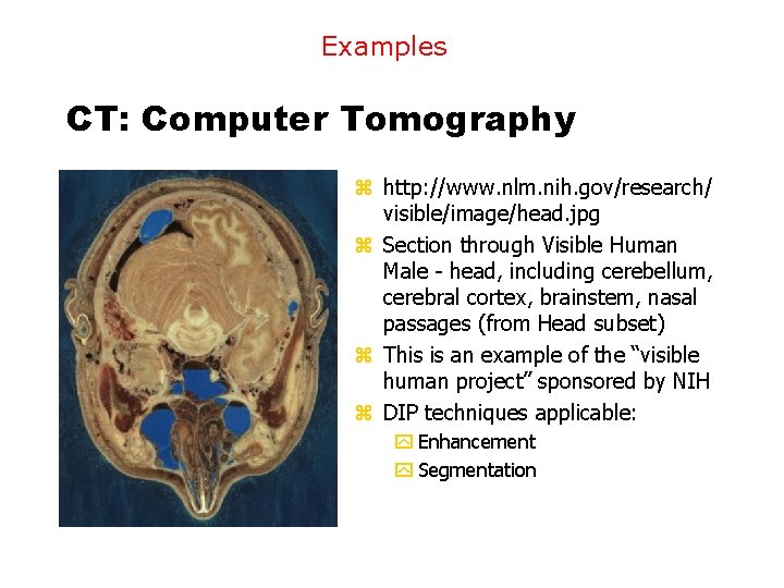
Examples CT: Computer Tomography z http: //www. nlm. nih. gov/research/ visible/image/head. jpg z Section through Visible Human Male - head, including cerebellum, cerebral cortex, brainstem, nasal passages (from Head subset) z This is an example of the “visible human project” sponsored by NIH z DIP techniques applicable: y Enhancement y Segmentation

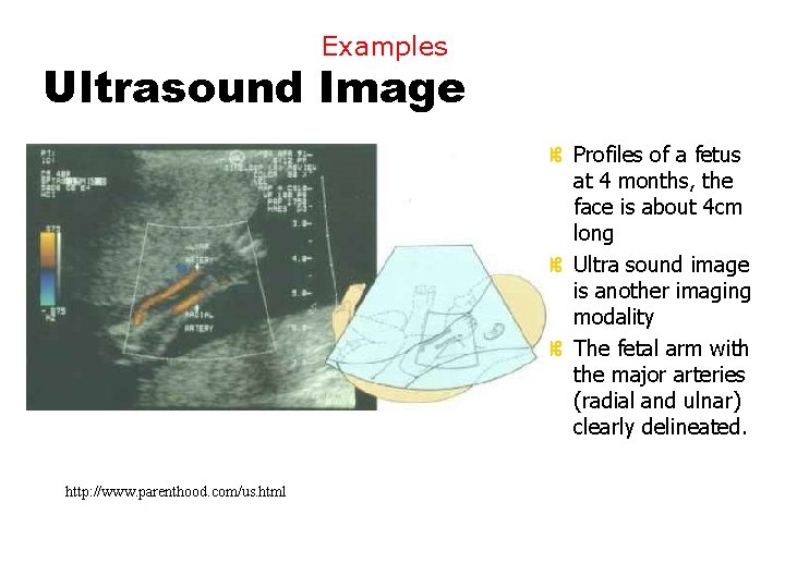
Examples Ultrasound Image z Profiles of a fetus at 4 months, the face is about 4 cm long z Ultra sound image is another imaging modality z The fetal arm with the major arteries (radial and ulnar) clearly delineated. http: //www. parenthood. com/us. html

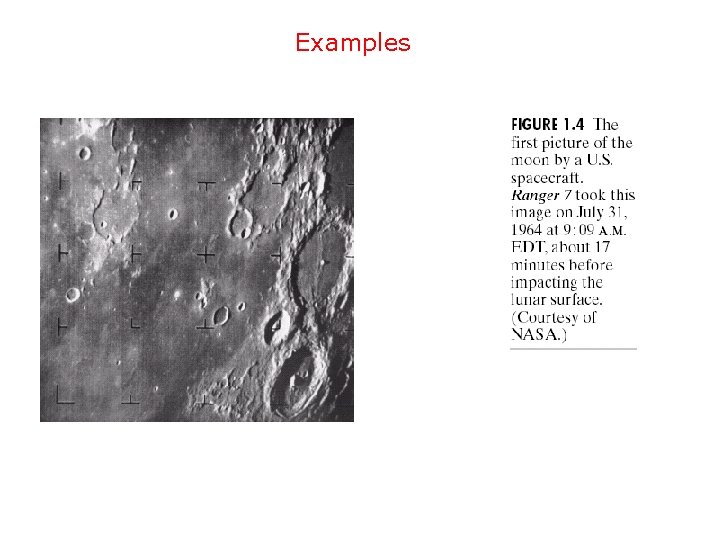
Examples

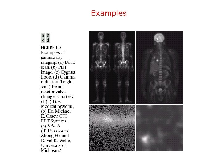
Examples

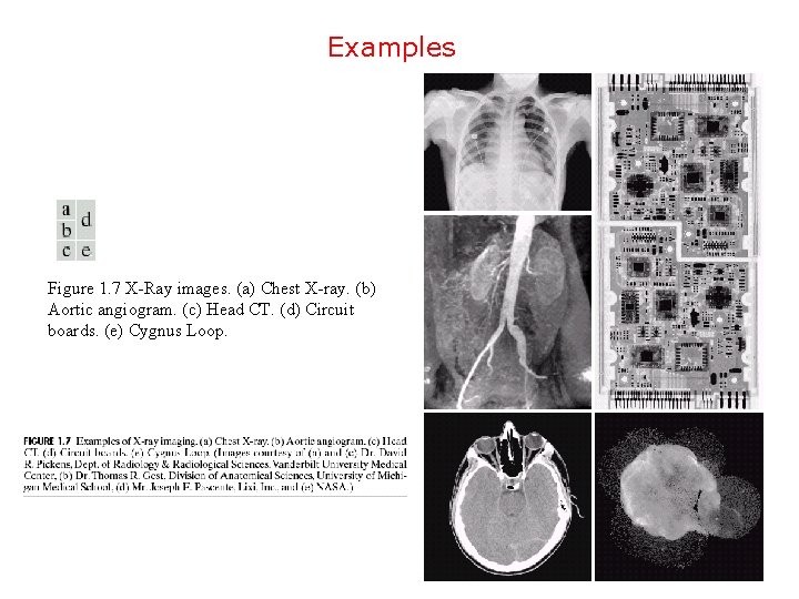
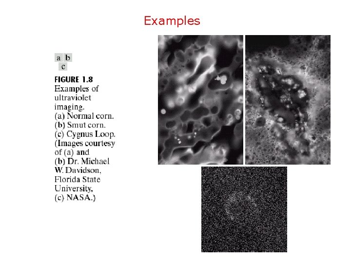
Examples Figure 1. 7 X-Ray images. (a) Chest X-ray. (b) Aortic angiogram. (c) Head CT. (d) Circuit boards. (e) Cygnus Loop.

Examples

Why Digital Image Processing (DIP)? z One picture worth 1000 words! z Support visual communication z Facilitate inspection, diagnosis of complex systems y Human body y Manufacturing z Entertainment z Keep record, history z Managing multimedia information z Security, y monitoring, y watermarking, etc

Digital Image Processing z Human vision - perceive and understand world z Computer vision, Image Understanding / Interpretation, Image processing. y 3 D world -> sensors (TV cameras) -> 2 D images y Dimension reduction -> loss of information z low level image processing xtransform of one image to another z high level image understanding xknowledge based - imitate human cognition xmake decisions according to information in image

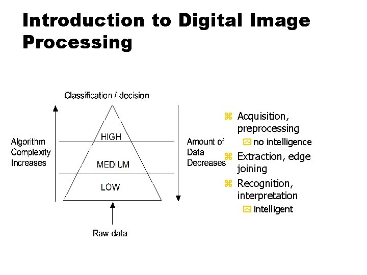
Introduction to Digital Image Processing z Acquisition, preprocessing y no intelligence z Extraction, edge joining z Recognition, interpretation y intelligent

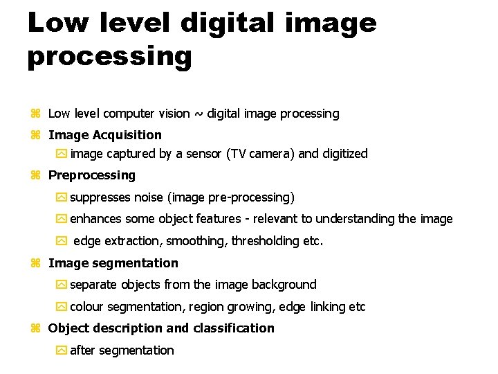
Low level digital image processing z Low level computer vision ~ digital image processing z Image Acquisition y image captured by a sensor (TV camera) and digitized z Preprocessing y suppresses noise (image pre-processing) y enhances some object features - relevant to understanding the image y edge extraction, smoothing, thresholding etc. z Image segmentation y separate objects from the image background y colour segmentation, region growing, edge linking etc z Object description and classification y after segmentation

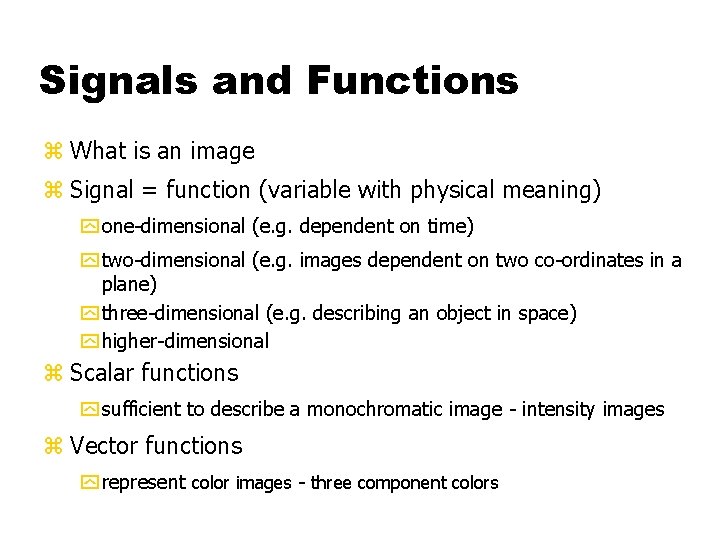
Signals and Functions z What is an image z Signal = function (variable with physical meaning) y one-dimensional (e. g. dependent on time) y two-dimensional (e. g. images dependent on two co-ordinates in a plane) y three-dimensional (e. g. describing an object in space) y higher-dimensional z Scalar functions y sufficient to describe a monochromatic image - intensity images z Vector functions y represent color images - three component colors

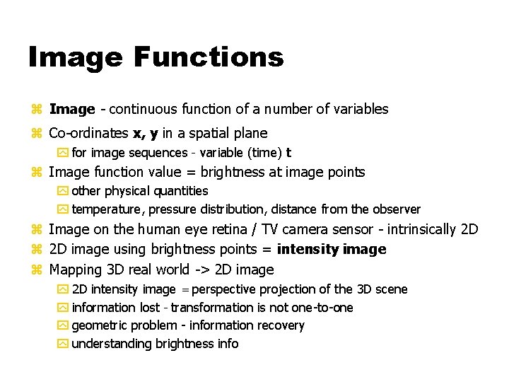
Image Functions z Image - continuous function of a number of variables z Co-ordinates x, y in a spatial plane y for image sequences - variable (time) t z Image function value = brightness at image points y other physical quantities y temperature, pressure distribution, distance from the observer z Image on the human eye retina / TV camera sensor - intrinsically 2 D z 2 D image using brightness points = intensity image z Mapping 3 D real world -> 2 D image y 2 D intensity image = perspective projection of the 3 D scene y information lost - transformation is not one-to-one y geometric problem - information recovery y understanding brightness info

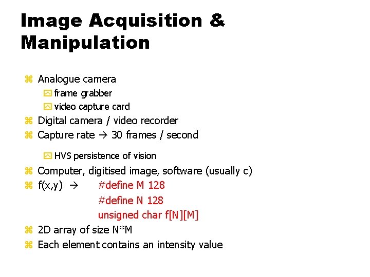
Image Acquisition & Manipulation z Analogue camera y frame grabber y video capture card z Digital camera / video recorder z Capture rate 30 frames / second y HVS persistence of vision z Computer, digitised image, software (usually c) z f(x, y) #define M 128 #define N 128 unsigned char f[N][M] z 2 D array of size N*M z Each element contains an intensity value

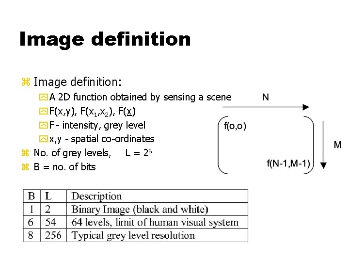
Image definition z Image definition: y A 2 D function obtained by sensing a scene y F(x, y), F(x 1, x 2), F(x) y F - intensity, grey level y x, y - spatial co-ordinates z No. of grey levels, L = 2 B z B = no. of bits

Brightness and 2 D images z Brightness dependent several factors y object surface reflectance properties x surface material, microstructure and marking y illumination properties y object surface orientation with respect to a viewer and light source z Some Scientific / technical disciplines work with 2 D images directly y image of flat specimen viewed by a microscope with transparent illumination y character drawn on a sheet of paper y image of a fingerprint

Monochromatic images z Image processing - static images - time t is constant z Monochromatic static image - continuous image function f(x, y) y arguments - two co-ordinates (x, y) z Digital image functions - represented by matrices y co-ordinates = integer numbers y Cartesian (horizontal x axis, vertical y axis) y. OR (row, column) matrices z Monochromatic image function range y lowest value - black y highest value - white z Limited brightness values = gray levels

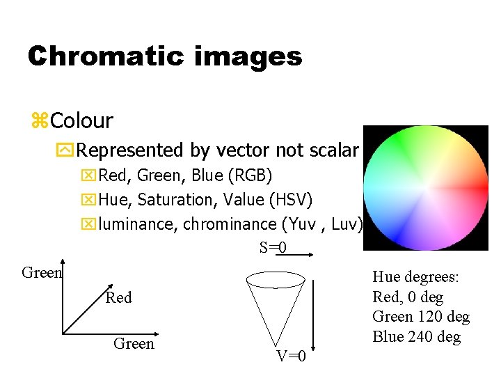
Chromatic images z. Colour y. Represented by vector not scalar x. Red, Green, Blue (RGB) x. Hue, Saturation, Value (HSV) xluminance, chrominance (Yuv , Luv) S=0 Green Hue degrees: Red, 0 deg Green 120 deg Blue 240 deg Red Green V=0

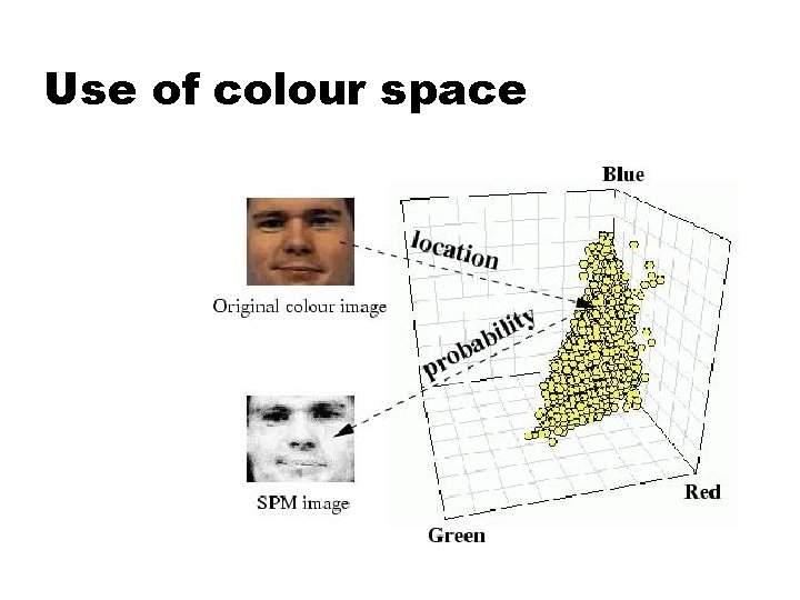
Use of colour space

Image quality z Quality of digital image proportional to: yspatial resolution xproximity of image samples in image plane yspectral resolution xbandwidth of light frequencies captured by sensor yradiometric resolution xnumber of distinguishable gray levels ytime resolution xinterval between time samples at which images captured

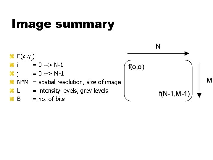
Image summary z z z F(xi, yj) i = 0 --> N-1 j = 0 --> M-1 N*M = spatial resolution, size of image L = intensity levels, grey levels B = no. of bits

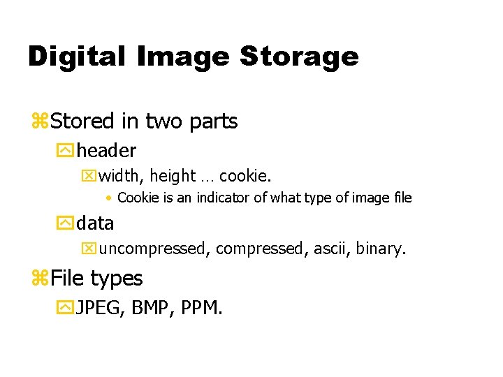
Digital Image Storage z. Stored in two parts yheader xwidth, height … cookie. • Cookie is an indicator of what type of image file ydata xuncompressed, ascii, binary. z. File types y. JPEG, BMP, PPM.

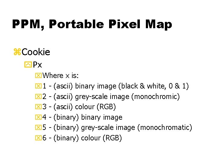
PPM, Portable Pixel Map z. Cookie y. Px x. Where x is: x 1 - (ascii) binary image (black & white, 0 & 1) x 2 - (ascii) grey-scale image (monochromic) x 3 - (ascii) colour (RGB) x 4 - (binary) binary image x 5 - (binary) grey-scale image (monochromatic) x 6 - (binary) colour (RGB)

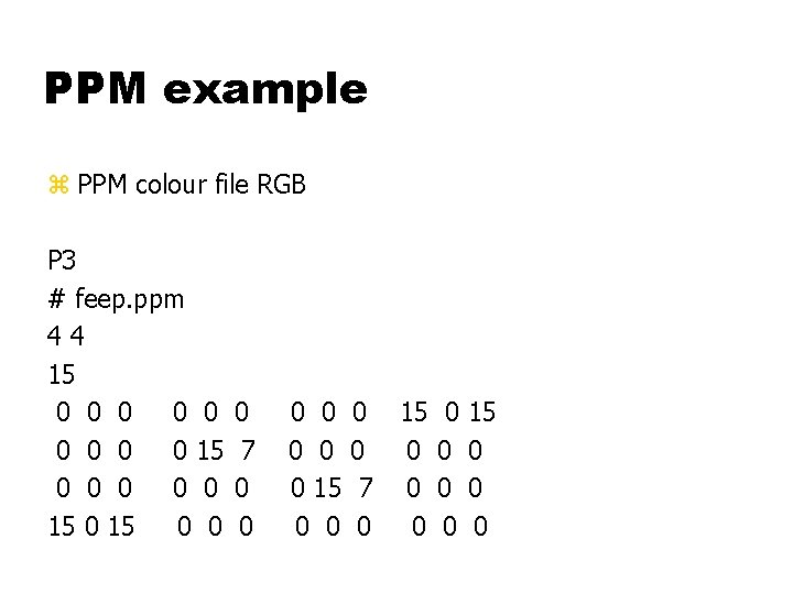
PPM example z PPM colour file RGB P 3 # feep. ppm 44 15 0 0 0 0 0 15 0 0 0 7 0 0 0 0 15 0 0 7 0 15 0 0 0

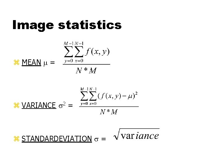
Image statistics z MEAN = z VARIANCE 2 = z STANDARDEVIATION =

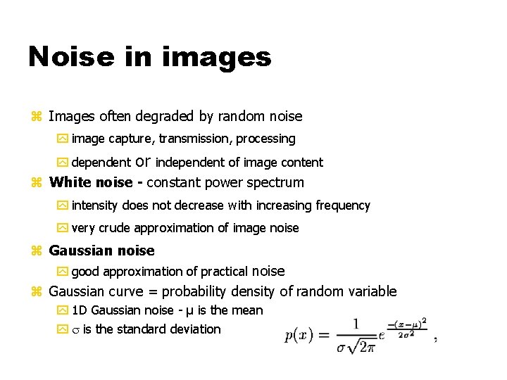
Noise in images z Images often degraded by random noise y image capture, transmission, processing y dependent or independent of image content z White noise - constant power spectrum y intensity does not decrease with increasing frequency y very crude approximation of image noise z Gaussian noise y good approximation of practical noise z Gaussian curve = probability density of random variable y 1 D Gaussian noise - µ is the mean y is the standard deviation

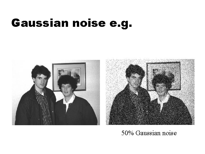
Gaussian noise e. g. 50% Gaussian noise

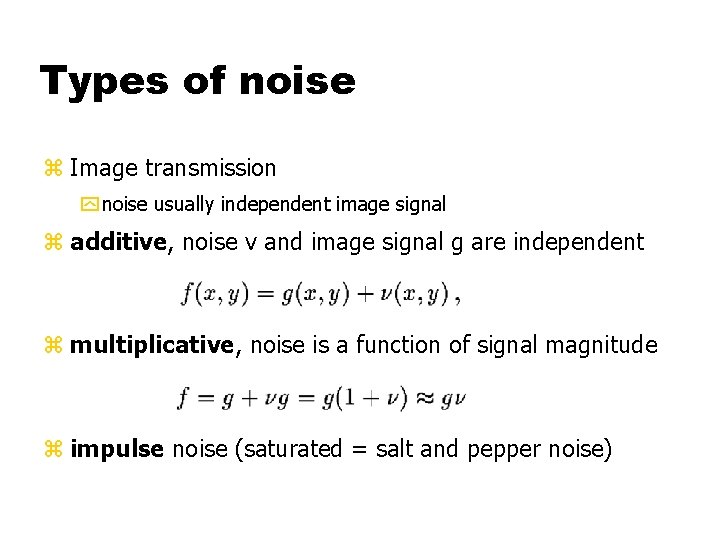
Types of noise z Image transmission y noise usually independent image signal z additive, noise v and image signal g are independent z multiplicative, noise is a function of signal magnitude z impulse noise (saturated = salt and pepper noise)

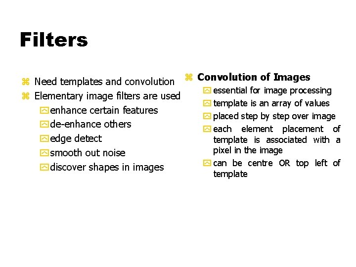
Filters z Need templates and convolution z Convolution of Images y essential for image processing z Elementary image filters are used y template is an array of values y enhance certain features y placed step by step over image y de-enhance others y each element placement of y edge detect template is associated with a pixel in the image y smooth out noise y can be centre OR top left of y discover shapes in images template

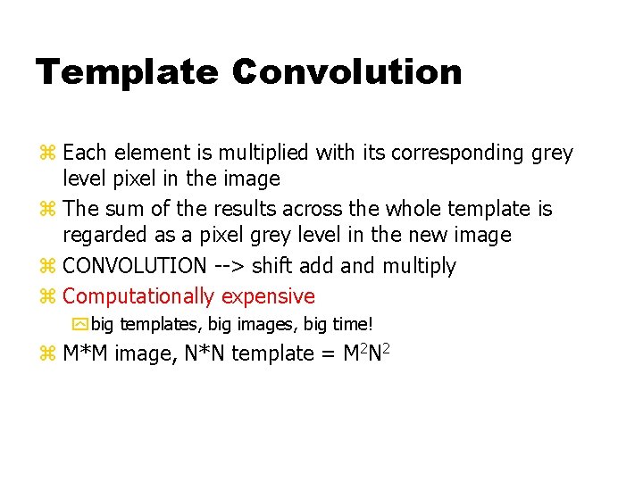
Template Convolution z Each element is multiplied with its corresponding grey level pixel in the image z The sum of the results across the whole template is regarded as a pixel grey level in the new image z CONVOLUTION --> shift add and multiply z Computationally expensive y big templates, big images, big time! z M*M image, N*N template = M 2 N 2

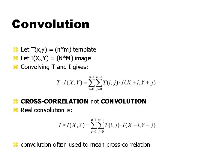
Convolution z Let T(x, y) = (n*m) template z Let I(X, , Y) = (N*M) image z Convolving T and I gives: z CROSS-CORRELATION not CONVOLUTION z Real convolution is: z convolution often used to mean cross-correlation

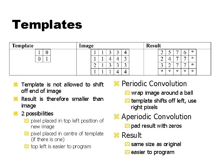
Templates z Template is not allowed to shift off end of image z Result is therefore smaller than image z 2 possibilities y pixel placed in top left position of new image y pixel placed in centre of template (if there is one) y top left is easier to program z Periodic Convolution y wrap image around a ball y template shifts off left, use right pixels z Aperiodic Convolution y pad result with zeros z Result y same size as original y easier to program

Filters z Need templates and convolution z Convolution of Images y essential for image processing z Elementary image filters are used y template is an array of values y enhance certain features y placed step by step over image y de-enhance others y each element placement of y edge detect template is associated with a pixel in the image y smooth out noise y can be centre OR top left of y discover shapes in images template

Template Convolution z Each element is multiplied with its corresponding grey level pixel in the image z The sum of the results across the whole template is regarded as a pixel grey level in the new image z CONVOLUTION --> shift add and multiply z Computationally expensive y big templates, big images, big time! z M*M image, N*N template = M 2 N 2

Templates z Template is not allowed to shift off end of image z Result is therefore smaller than image z 2 possibilities y pixel placed in top left position of new image y pixel placed in centre of template (if there is one) y top left is easier to program z Periodic Convolution y wrap image around a ball y template shifts off left, use right pixels z Aperiodic Convolution y pad result with zeros z Result y same size as original y easier to program

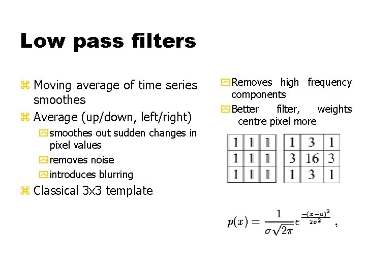
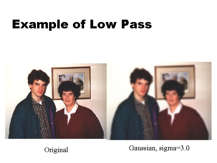
Low pass filters z Moving average of time series smoothes z Average (up/down, left/right) y smoothes out sudden changes in pixel values y removes noise y introduces blurring z Classical 3 x 3 template y Removes high frequency components y Better filter, weights centre pixel more

Example of Low Pass Original Gaussian, sigma=3. 0

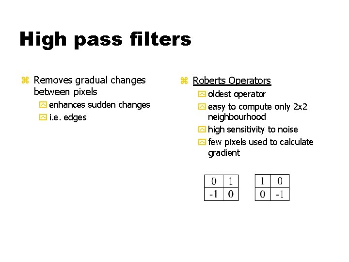
High pass filters z Removes gradual changes between pixels y enhances sudden changes y i. e. edges z Roberts Operators y oldest operator y easy to compute only 2 x 2 neighbourhood y high sensitivity to noise y few pixels used to calculate gradient

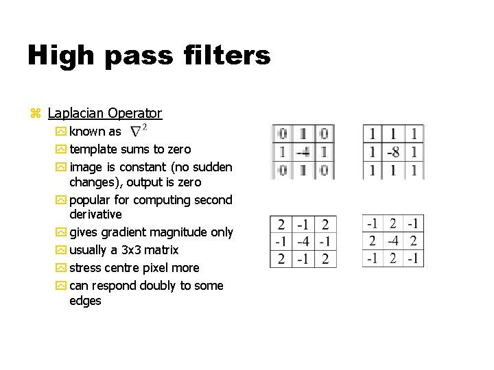
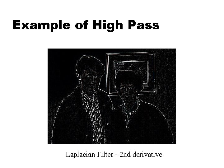
High pass filters z Laplacian Operator y known as y template sums to zero y image is constant (no sudden changes), output is zero y popular for computing second derivative y gives gradient magnitude only y usually a 3 x 3 matrix y stress centre pixel more y can respond doubly to some edges

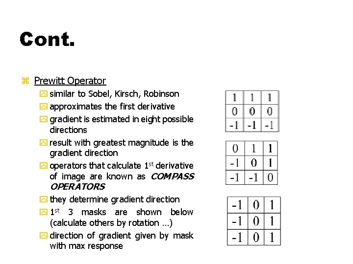
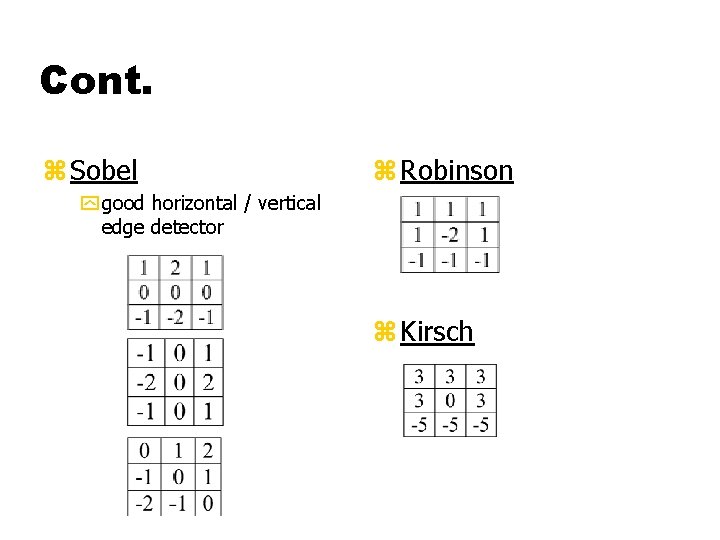
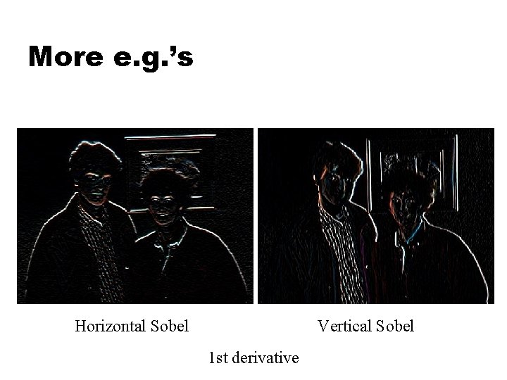
Cont. z Prewitt Operator y similar to Sobel, Kirsch, Robinson y approximates the first derivative y gradient is estimated in eight possible directions y result with greatest magnitude is the gradient direction y operators that calculate 1 st derivative of image are known as COMPASS OPERATORS y they determine gradient direction y 1 st 3 masks are shown below (calculate others by rotation …) y direction of gradient given by mask with max response

Cont. z Sobel z Robinson y good horizontal / vertical edge detector z Kirsch

Example of High Pass Laplacian Filter - 2 nd derivative

More e. g. ’s Horizontal Sobel Vertical Sobel 1 st derivative

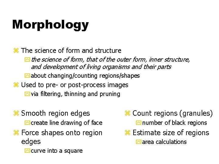
Morphology z The science of form and structure y the science of form, that of the outer form, inner structure, and development of living organisms and their parts y about changing/counting regions/shapes z Used to pre- or post-process images y via filtering, thinning and pruning z Smooth region edges z Count regions (granules) y create line drawing of face y number of black regions z Force shapes onto region edges z Estimate size of regions y curve into a square y area calculations

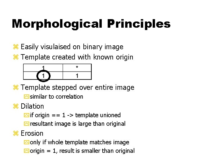
Morphological Principles z Easily visulaised on binary image z Template created with known origin z Template stepped over entire image y similar to correlation z Dilation y if origin == 1 -> template unioned y resultant image is large than original z Erosion y only if whole template matches image y origin = 1, result is smaller than original

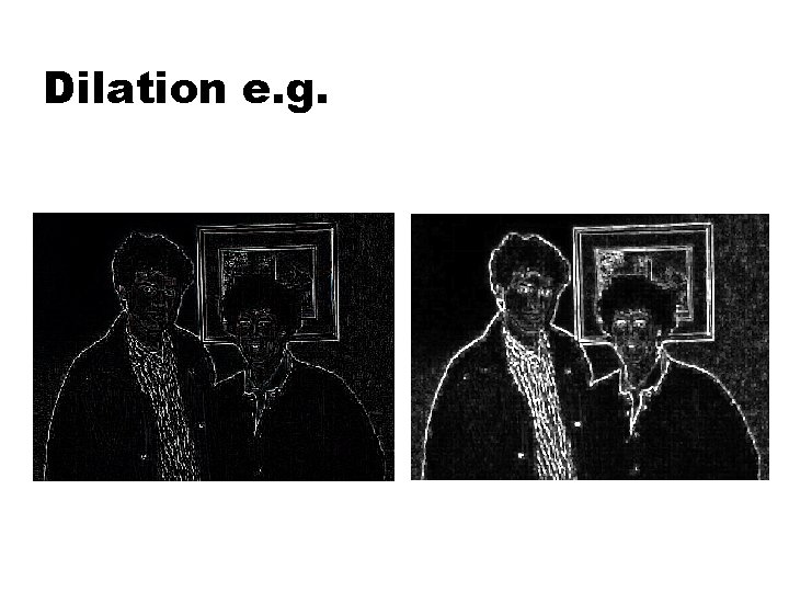
Dilation z Dilation (Minkowski addition) yfills in valleys between spiky regions yincreases geometrical area of object yobjects are light (white in binary) ysets background pixels adjacent to object's contour to object's value ysmoothes small negative grey level regions

Dilation e. g.

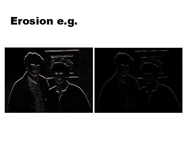
Erosion z Erosion (Minkowski subtraction) yremoves spiky edges yobjects are light (white in binary) ydecreases geometrical area of object ysets contour pixels of object to background value ysmoothes small positive grey level regions

Erosion e. g.