Introduction to ContinuousTime Markov Chains and Queueing Theory

Introduction to Continuous-Time Markov Chains and Queueing Theory Thrasyvoulos Spyropoulos / spyropou@eurecom. fr Eurecom, Sophia-Antipolis

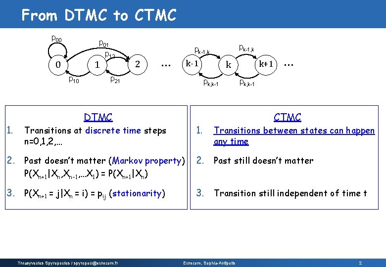
From DTMC to CTMC p 00 p 01 p 12 1 0 p 10 1. pk-1, k 2 … k-1 p 21 pk, k-1 DTMC 1. Transitions at discrete time steps n=0, 1, 2, … 2. Past doesn’t matter (Markov property) k+1 k … pk, k-1 CTMC Transitions between states can happen any time 2. Past still doesn’t matter P(Xn+1|Xn, Xn-1, …X 1) = P(Xn+1|Xn) 3. P(Xn+1 = j|Xn = i) = pij (stationarity) Thrasyvoulos Spyropoulos / spyropou@eurecom. fr 3. Transition still independent of time t Eurecom, Sophia-Antipolis 2

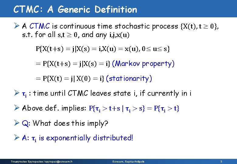
CTMC: A Generic Definition Ø A CTMC is continuous time stochastic process {X(t), t ≥ 0}, s. t. for all s, t ≥ 0, and any i, j, x(u) P{X(t+s) = j|X(s) = i, X(u) = x(u), 0≤ u≤ s} = P{X(t+s) = j|X(s) = i} (Markov property) = P{X(t) = j| X(0) = i} (stationarity) Ø τi : time until CTMC leaves state i, if currently in i Ø Above def. implies: P{τi > t+s | τi > s} = P{τi > t} Ø Q: What does this imply? Ø A: τi is exponentially distributed! Thrasyvoulos Spyropoulos / spyropou@eurecom. fr Eurecom, Sophia-Antipolis 3

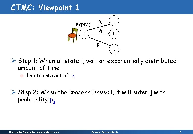
CTMC: Viewpoint 1 exp(vi) i pij pik pil j k l Ø Step 1: When at state i, wait an exponentially distributed amount of time v denote rate out of: vi Ø Step 2: When the process leaves i, it will enter j with probability pij Thrasyvoulos Spyropoulos / spyropou@eurecom. fr Eurecom, Sophia-Antipolis 4

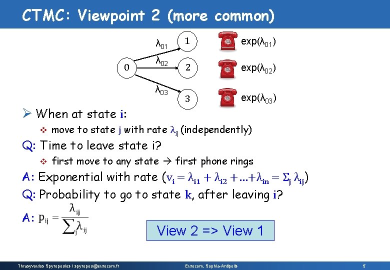
CTMC: Viewpoint 2 (more common) λ 01 0 λ 02 λ 03 1 exp(λ 01) 2 exp(λ 02) 3 exp(λ 03) Ø When at state i: v move to state j with rate λij (independently) Q: Time to leave state i? v first move to any state first phone rings A: Exponential with rate (vi = λi 1 + λi 2 +…+λin = Σj λij) Q: Probability to go to state k, after leaving i? A: Thrasyvoulos Spyropoulos / spyropou@eurecom. fr View 2 => View 1 Eurecom, Sophia-Antipolis 5

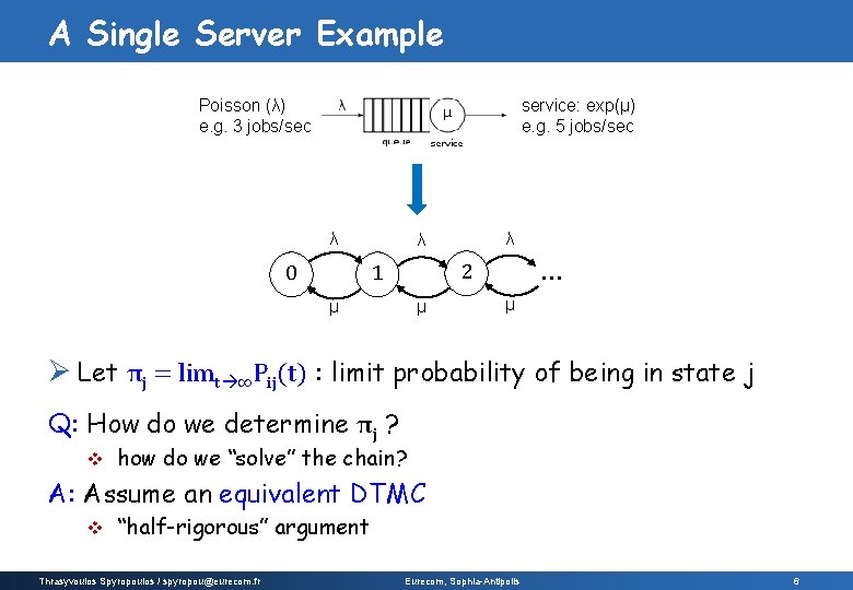
A Single Server Example Poisson (λ) e. g. 3 jobs/sec service: exp(μ) e. g. 5 jobs/sec λ 2 1 0 λ λ μ μ … μ Ø Let πj = limt ∞Pij(t) : limit probability of being in state j Q: How do we determine πj ? v how do we “solve” the chain? A: Assume an equivalent DTMC v “half-rigorous” argument Thrasyvoulos Spyropoulos / spyropou@eurecom. fr Eurecom, Sophia-Antipolis 6

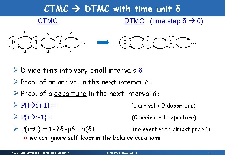
CTMC DTMC with time unit δ DTMC (time step δ 0) CTMC λ 2 1 0 μ λ λ μ λδ+o(δ) μ 2 1 0 … λδ+o(δ) μδ+o(δ) … μδ+o(δ) Ø Divide time into very small intervals δ Ø Prob. of an arrival in the next interval δ : λδ + o(δ) Ø Prob. of a departure in the next interval δ : μδ + o(δ) Ø P{i i+1} = λδ (1 -μδ) = λδ + o(δ) (1 arrival + 0 departure) Ø P{i i-1} = μδ (1 - λδ) = μδ + o(δ) (0 arrival + 1 departure) Ø P{i i} = 1 - λδ -μδ +o(δ) (no event with almost prob 1) v we can ignore self-loops in the balance equations Thrasyvoulos Spyropoulos / spyropou@eurecom. fr Eurecom, Sophia-Antipolis 7

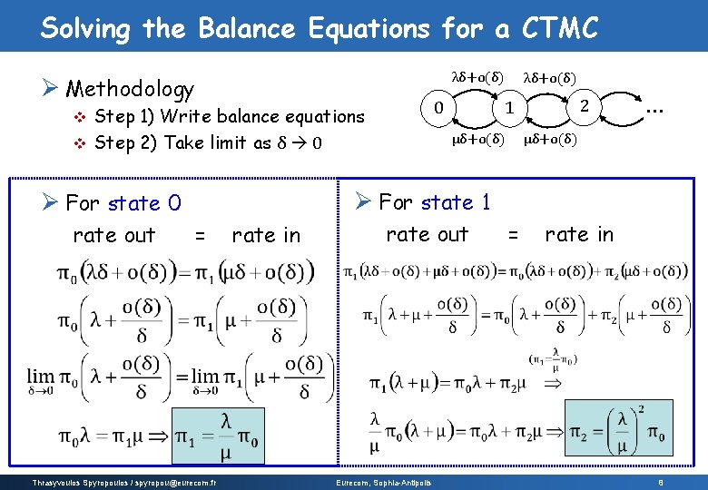
Solving the Balance Equations for a CTMC λδ+o(δ) Ø Methodology μδ+o(δ) … μδ+o(δ) Ø For state 1 Ø For state 0 rate out 2 1 0 Step 1) Write balance equations v Step 2) Take limit as δ 0 v λδ+o(δ) = Thrasyvoulos Spyropoulos / spyropou@eurecom. fr rate in rate out Eurecom, Sophia-Antipolis = rate in 8

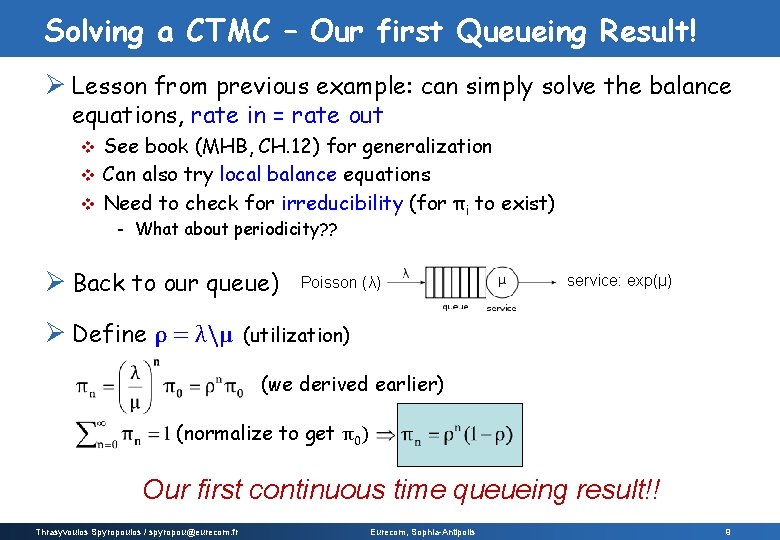
Solving a CTMC – Our first Queueing Result! Ø Lesson from previous example: can simply solve the balance equations, rate in = rate out See book (MHB, CH. 12) for generalization v Can also try local balance equations v Need to check for irreducibility (for πi to exist) v - What about periodicity? ? Ø Back to our queue) Ø Define ρ = λμ Poisson (λ) service: exp(μ) (utilization) (we derived earlier) (normalize to get π0) Our first continuous time queueing result!! Thrasyvoulos Spyropoulos / spyropou@eurecom. fr Eurecom, Sophia-Antipolis 9

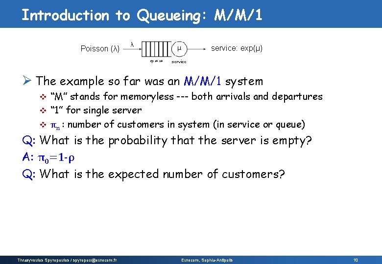
Introduction to Queueing: M/M/1 Poisson (λ) service: exp(μ) Ø The example so far was an M/M/1 system “M” stands for memoryless --- both arrivals and departures v “ 1” for single server v πn : number of customers in system (in service or queue) v Q: What is the probability that the server is empty? A: π0=1 -ρ Q: What is the expected number of customers? A: Thrasyvoulos Spyropoulos / spyropou@eurecom. fr Eurecom, Sophia-Antipolis 10

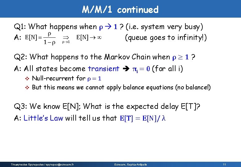
M/M/1 continued Q 1: What happens when ρ 1 ? (i. e. system very busy) A: (queue goes to infinity!) Q 2: What happens to the Markov Chain when ρ ≥ 1 ? A: All states become transient πi = 0 (for all i) Null-recurrent for ρ = 1 v But this means we cannot apply balance equations (no balance!) v Q 3: We know E[N]; What is the expected delay E[T]? A: Little’s Law will tell us that E[T] = E[N]/ λ Thrasyvoulos Spyropoulos / spyropou@eurecom. fr Eurecom, Sophia-Antipolis 11

Introduction to Queueing Theory Thrasyvoulos Spyropoulos / spyropou@eurecom. fr Eurecom, Sophia-Antipolis 12

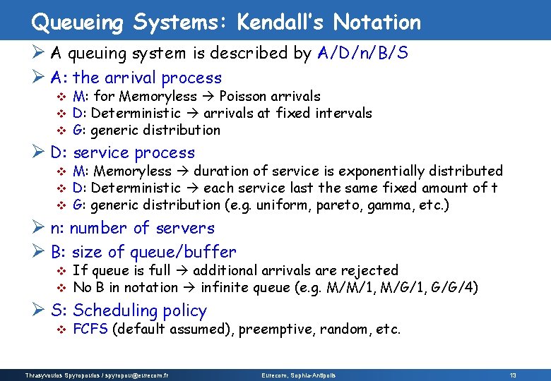
Queueing Systems: Kendall’s Notation Ø A queuing system is described by A/D/n/B/S Ø A: the arrival process v v v M: for Memoryless Poisson arrivals D: Deterministic arrivals at fixed intervals G: generic distribution Ø D: service process v v v M: Memoryless duration of service is exponentially distributed D: Deterministic each service last the same fixed amount of t G: generic distribution (e. g. uniform, pareto, gamma, etc. ) Ø n: number of servers Ø B: size of queue/buffer v v If queue is full additional arrivals are rejected No B in notation infinite queue (e. g. M/M/1, M/G/1, G/G/4) Ø S: Scheduling policy v FCFS (default assumed), preemptive, random, etc. Thrasyvoulos Spyropoulos / spyropou@eurecom. fr Eurecom, Sophia-Antipolis 13

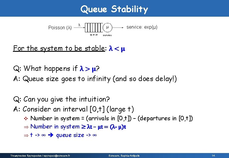
Queue Stability service: exp(μ) Poisson (λ) For the system to be stable: λ < μ Q: What happens if λ > μ? A: Queue size goes to infinity (and so does delay!) Q: Can you give the intuition? A: Consider an interval [0, t] (large t) Number in system = (arrivals in [0, t]) – (departures in [0, t]) Þ Number in system ≥ λt – μt = (λ- μ)t Þ t -> ∞ queue size -> ∞ v Thrasyvoulos Spyropoulos / spyropou@eurecom. fr Eurecom, Sophia-Antipolis 14

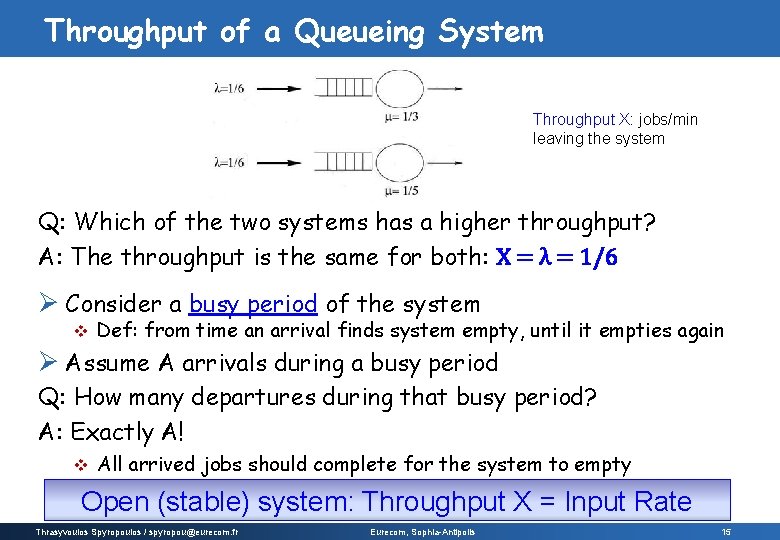
Throughput of a Queueing System Throughput X: jobs/min leaving the system Q: Which of the two systems has a higher throughput? A: The throughput is the same for both: X = λ = 1/6 Ø Consider a busy period of the system v Def: from time an arrival finds system empty, until it empties again Ø Assume A arrivals during a busy period Q: How many departures during that busy period? A: Exactly A! v All arrived jobs should complete for the system to empty Open (stable) system: Throughput X = Input Rate Thrasyvoulos Spyropoulos / spyropou@eurecom. fr Eurecom, Sophia-Antipolis 15

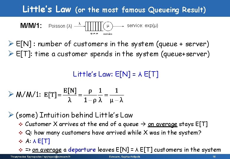
Little’s Law M/M/1: Poisson (λ) (or the most famous Queueing Result) service: exp(μ) Ø E[N] : number of customers in the system (queue + server) Ø E[T]: time a customer spends in the system (queue+server) Little’s Law: E[N] = λ E[T] Ø M/M/1: Ø (some) Intuition behind Little’s Law Customer X arrives at the end of a queue on average stays E[T] v Q: how many customers have arrived while X was in the system? v A: λ E[T] v => on average a departure leaves E[N] = λ E[T] customers in the system v Thrasyvoulos Spyropoulos / spyropou@eurecom. fr Eurecom, Sophia-Antipolis 16

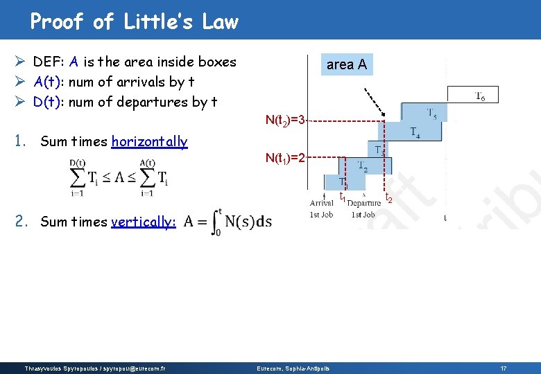
Proof of Little’s Law Ø DEF: A is the area inside boxes Ø A(t): num of arrivals by t Ø D(t): num of departures by t area A N(t 2)=3 1. Sum times horizontally N(t 1)=2 t 1 t 2 2. Sum times vertically: Thrasyvoulos Spyropoulos / spyropou@eurecom. fr Eurecom, Sophia-Antipolis 17

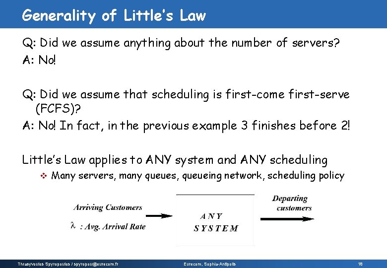
Generality of Little’s Law Q: Did we assume anything about the number of servers? A: No! Q: Did we assume that scheduling is first-come first-serve (FCFS)? A: No! In fact, in the previous example 3 finishes before 2! Little’s Law applies to ANY system and ANY scheduling v Many servers, many queues, queueing network, scheduling policy Thrasyvoulos Spyropoulos / spyropou@eurecom. fr Eurecom, Sophia-Antipolis 18

Little’s Law: Additional Results Q: What about E[TQ]? v number of jobs in queue – not server(s) A: λE[TQ] = E[NQ] (similar proof) Q: What about ρ (number of customers in service)? A: λE[S] = ρ ρ = λ/μ Q: What is ρ? A: System utilization -> fraction of time server(s) is busy (time average) A: Ergodicity Prob{server is busy at a random time} (ensemble average) Thrasyvoulos Spyropoulos / spyropou@eurecom. fr Eurecom, Sophia-Antipolis 19

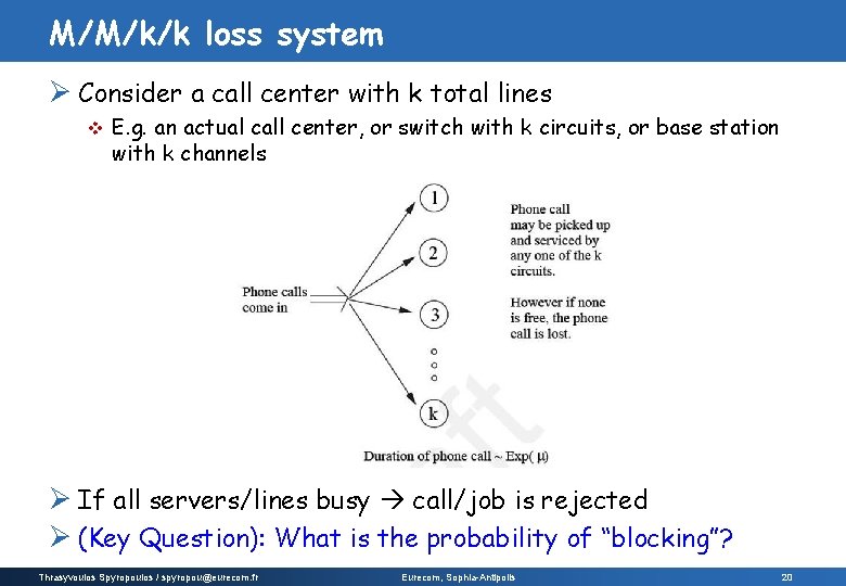
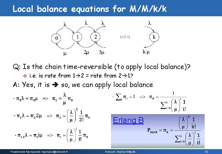
M/M/k/k loss system Ø Consider a call center with k total lines v E. g. an actual call center, or switch with k circuits, or base station with k channels Ø If all servers/lines busy call/job is rejected Ø (Key Question): What is the probability of “blocking”? Thrasyvoulos Spyropoulos / spyropou@eurecom. fr Eurecom, Sophia-Antipolis 20

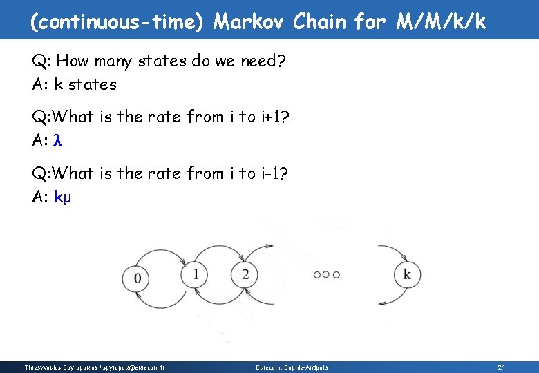
(continuous-time) Markov Chain for M/M/k/k Q: How many states do we need? A: k states Q: What is the rate from i to i+1? A: λ Q: What is the rate from i to i-1? A: kμ Thrasyvoulos Spyropoulos / spyropou@eurecom. fr Eurecom, Sophia-Antipolis 21

Local balance equations for M/M/k/k Q: Is the chain time-reversible (to apply local balance)? v i. e. is rate from 1 2 = rate from 2 1? A: Yes, it is so, we can apply local balance Erlang B Thrasyvoulos Spyropoulos / spyropou@eurecom. fr Eurecom, Sophia-Antipolis 22

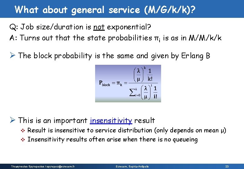
What about general service (M/G/k/k)? Q: Job size/duration is not exponential? A: Turns out that the state probabilities πi is as in M/M/k/k Ø The block probability is the same and given by Erlang B Ø This is an important insensitivity result Result is insensitive to service distribution (only depends on mean μ) v Insensitivity results often arise when there is no queueing v Thrasyvoulos Spyropoulos / spyropou@eurecom. fr Eurecom, Sophia-Antipolis 23

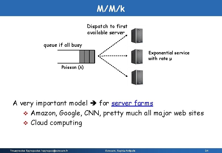
M/M/k Dispatch to first available server queue if all busy Exponential service with rate μ Poisson (λ) A very important model for server farms v Amazon, Google, CNN, pretty much all major web sites v Cloud computing Thrasyvoulos Spyropoulos / spyropou@eurecom. fr Eurecom, Sophia-Antipolis 24

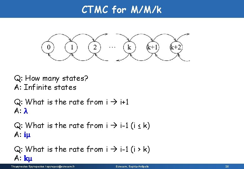
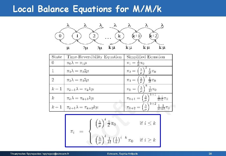
CTMC for M/M/k … Q: How many states? A: Infinite states Q: What is the rate from i i+1 A: λ Q: What is the rate from i i-1 (i ≤ k) A: iμ Q: What is the rate from i i-1 (i > k) A: kμ Thrasyvoulos Spyropoulos / spyropou@eurecom. fr Eurecom, Sophia-Antipolis 25

Local Balance Equations for M/M/k … Thrasyvoulos Spyropoulos / spyropou@eurecom. fr Eurecom, Sophia-Antipolis 26

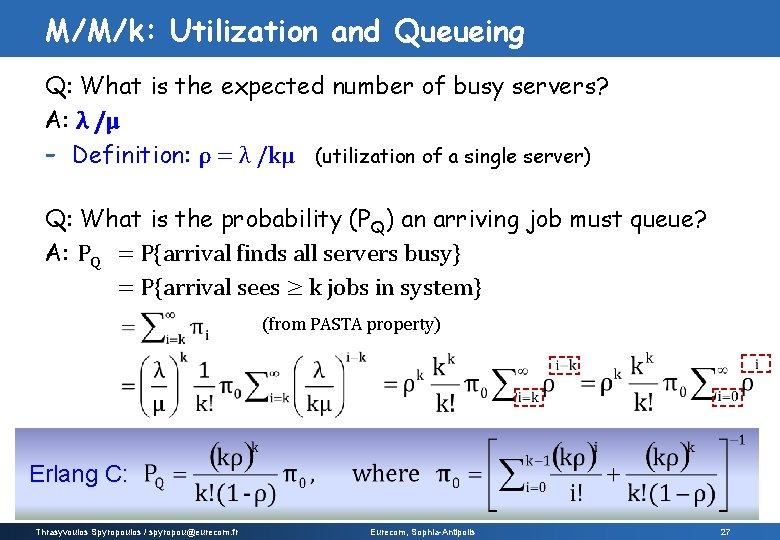
M/M/k: Utilization and Queueing Q: What is the expected number of busy servers? A: λ /μ - Definition: ρ = λ /kμ (utilization of a single server) Q: What is the probability (PQ) an arriving job must queue? A: PQ = P{arrival finds all servers busy} = P{arrival sees ≥ k jobs in system} (from PASTA property) Erlang C: Thrasyvoulos Spyropoulos / spyropou@eurecom. fr Eurecom, Sophia-Antipolis 27

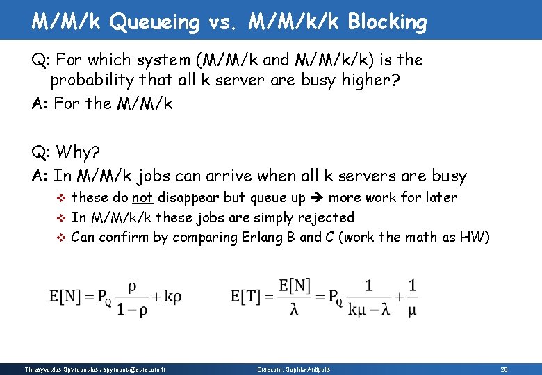
M/M/k Queueing vs. M/M/k/k Blocking Q: For which system (M/M/k and M/M/k/k) is the probability that all k server are busy higher? A: For the M/M/k Q: Why? A: In M/M/k jobs can arrive when all k servers are busy these do not disappear but queue up more work for later v In M/M/k/k these jobs are simply rejected v Can confirm by comparing Erlang B and C (work the math as HW) v Thrasyvoulos Spyropoulos / spyropou@eurecom. fr Eurecom, Sophia-Antipolis 28

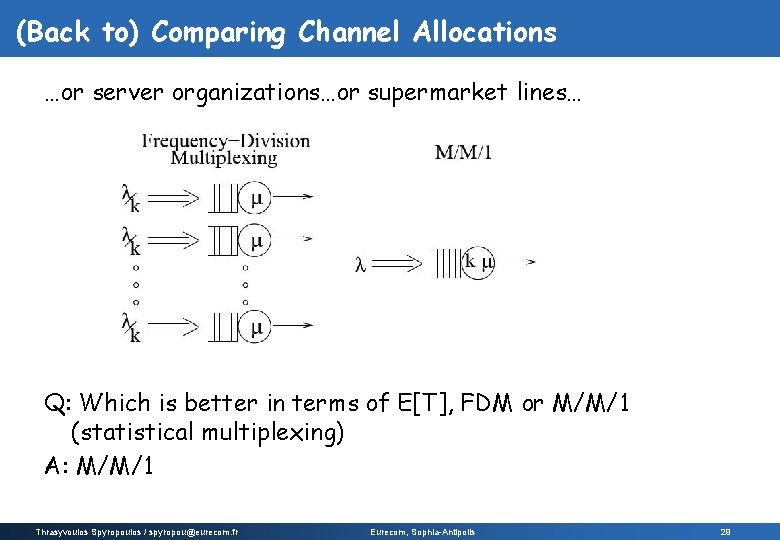
(Back to) Comparing Channel Allocations …or server organizations…or supermarket lines… Q: Which is better in terms of E[T], FDM or M/M/1 (statistical multiplexing) A: M/M/1 E[TFDM] = k/(kμ-λ) but E[TM/M/1] = 1/(kμ-λ) Thrasyvoulos Spyropoulos / spyropou@eurecom. fr Eurecom, Sophia-Antipolis 29

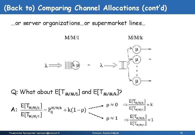
(Back to) Comparing Channel Allocations (cont’d) …or server organizations…or supermarket lines… Q: What about E[TM/M/1] and E[TM/M/k]? A: ρ≈0 ρ≈1 Thrasyvoulos Spyropoulos / spyropou@eurecom. fr Eurecom, Sophia-Antipolis 30