Introduction to Connectivity PPI and SEM Carmen Tur

Introduction to Connectivity: PPI and SEM Carmen Tur Maria Joao Rosa Methods for Dummies 2009/10 24 th February, UCL, London

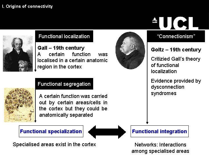
I. Origins of connectivity Functional localization Gall – 19 th century A certain function was localised in a certain anatomic region in the cortex Functional segregation A certain function was carried out by certain areas/cells in the cortex but they could be anatomically separated Functional specialization Specialised areas exist in the cortex “Connectionism” Goltz – 19 th century Critizied Gall’s theory of functional localization Evidence provided by dysconnection syndromes Functional integration Networks: Interactions among specialised areas

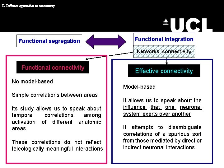
II. Different approaches to connectivity Functional segregation Functional integration Networks -connectivity Functional connectivity No model-based Simple correlations between areas Its study allows us to speak about temporal correlations among activation of different anatomic areas These correlations do not reflect teleologically meaningful interactions Effective connectivity Model-based It allows us to speak about the influence that one neuronal system exerts over another It attempts to disambiguate correlations of a spurious sort from those mediated by direct or indirect neuronal interactions

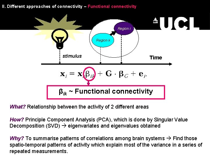
II. Different approaches of connectivity – Functional connectivity Region i Region k stimulus Time βik ~ Functional connectivity What? Relationship between the activity of 2 different areas How? Principle Component Analysis (PCA), which is done by Singular Value Decomposition (SVD) eigenvariates and eigenvalues obtained Why? To summarise patterns of correlations among brain systems Find those spatio-temporal patterns of activity which explain most of the variance in a series of repeated measurements.

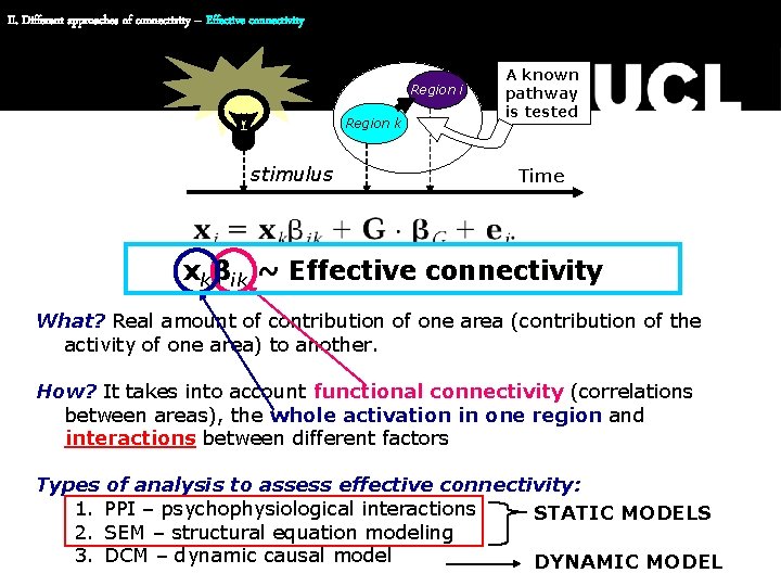
II. Different approaches of connectivity – Effective connectivity Region i Region k stimulus A known pathway is tested Time xkβik ~ Effective connectivity What? Real amount of contribution of one area (contribution of the activity of one area) to another. How? It takes into account functional connectivity (correlations between areas), the whole activation in one region and interactions between different factors Types of analysis to assess effective connectivity: 1. PPI – psychophysiological interactions STATIC MODELS 2. SEM – structural equation modeling 3. DCM – dynamic causal model DYNAMIC MODEL

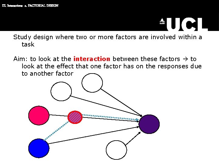
III. Interactions a. FACTORIAL DESIGN Study design where two or more factors are involved within a task Aim: to look at the interaction between these factors to look at the effect that one factor has on the responses due to another factor

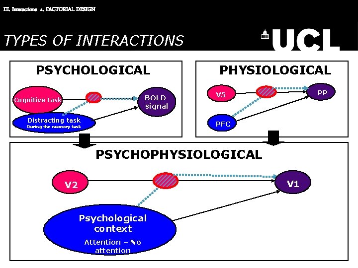
III. Interactions a. FACTORIAL DESIGN TYPES OF INTERACTIONS PSYCHOLOGICAL BOLD signal Cognitive task Distracting task PHYSIOLOGICAL PP V 5 PFC During the memory task PSYCHOPHYSIOLOGICAL V 1 V 2 Psychological context Attention – No attention

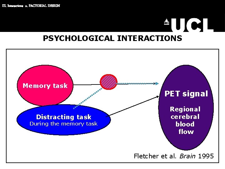
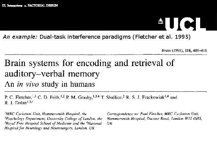
III. Interactions a. FACTORIAL DESIGN PSYCHOLOGICAL INTERACTIONS Memory task Distracting task During the memory task PET signal Regional cerebral blood flow Fletcher et al. Brain 1995

III. Interactions a. FACTORIAL DESIGN An example: Dual-task interference paradigms (Fletcher et al. 1995)

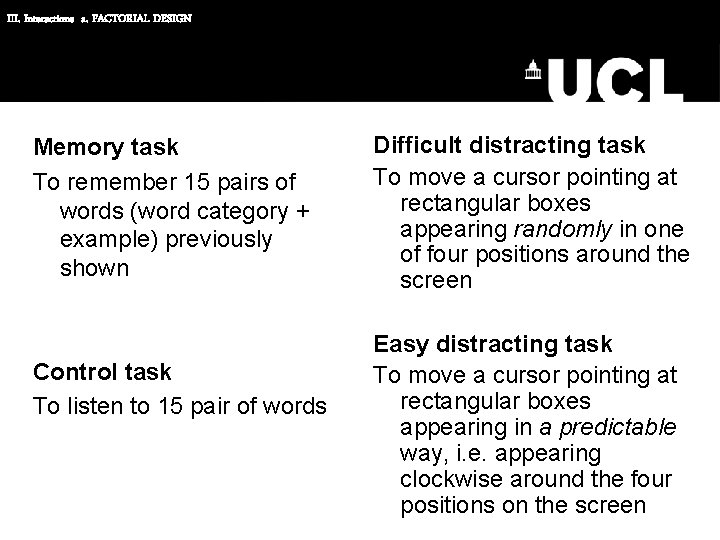
III. Interactions a. FACTORIAL DESIGN Memory task To remember 15 pairs of words (word category + example) previously shown Control task To listen to 15 pair of words Difficult distracting task To move a cursor pointing at rectangular boxes appearing randomly in one of four positions around the screen Easy distracting task To move a cursor pointing at rectangular boxes appearing in a predictable way, i. e. appearing clockwise around the four positions on the screen

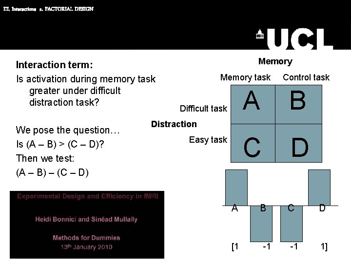
III. Interactions a. FACTORIAL DESIGN Interaction term: Is activation during memory task greater under difficult distraction task? We pose the question… Is (A – B) > (C – D)? Then we test: (A – B) – (C – D) Memory task Difficult task Control task A B C D Distraction Easy task A [1 B -1 C -1 D 1]

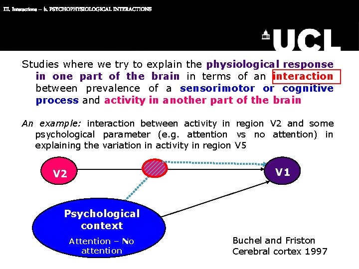
III. Interactions – b. PSYCHOPHYSIOLOGICAL INTERACTIONS Studies where we try to explain the physiological response in one part of the brain in terms of an interaction between prevalence of a sensorimotor or cognitive process and activity in another part of the brain An example: interaction between activity in region V 2 and some psychological parameter (e. g. attention vs no attention) in explaining the variation in activity in region V 5 V 1 V 2 Psychological context Attention – No attention Buchel and Friston Cerebral cortex 1997

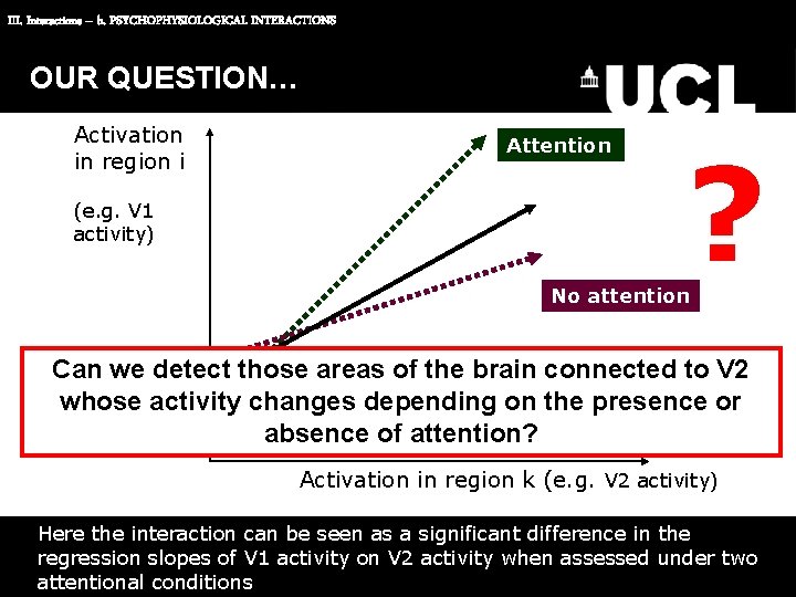
III. Interactions – b. PSYCHOPHYSIOLOGICAL INTERACTIONS OUR QUESTION… Activation in region i (e. g. V 1 activity) Attention ? No attention Can we detect those areas of the brain connected to V 2 whose activity changes depending on the presence or absence of attention? Activation in region k (e. g. V 2 activity) Here the interaction can be seen as a significant difference in the regression slopes of V 1 activity on V 2 activity when assessed under two attentional conditions

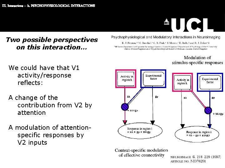
III. Interactions – b. PSYCHOPHYSIOLOGICAL INTERACTIONS Two possible perspectives on this interaction… We could have that V 1 activity/response reflects: A change of the contribution from V 2 by attention A modulation of attentionspecific responses by V 2 inputs

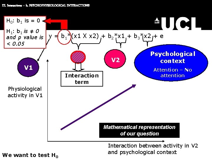
III. Interactions – b. PSYCHOPHYSIOLOGICAL INTERACTIONS H 0: b 1 is = 0 H 1: b 1 is ≠ 0 and p value is y = b 1*(x 1 X x 2) + b 2*x 1 + b 3*x 2 + e < 0. 05 V 2 V 1 Interaction term Psychological context Attention – No attention Physiological activity in V 1 Mathematical representation of our question We want to test H 0 Interaction between activity in V 2 and psychological context

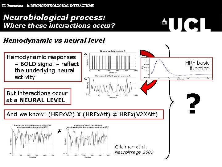
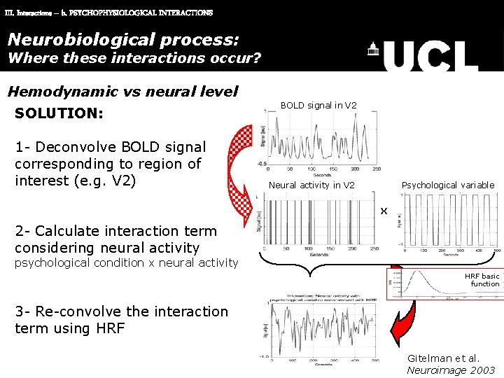
III. Interactions – b. PSYCHOPHYSIOLOGICAL INTERACTIONS Neurobiological process: Where these interactions occur? Hemodynamic vs neural level Hemodynamic responses – BOLD signal – reflect the underlying neural activity HRF basic function But interactions occur at a NEURAL LEVEL And we know: (HRFx. V 2) X (HRFx. Att) ≠ HRFx(V 2 XAtt) ≠ Gitelman et al. Neuroimage 2003 ?

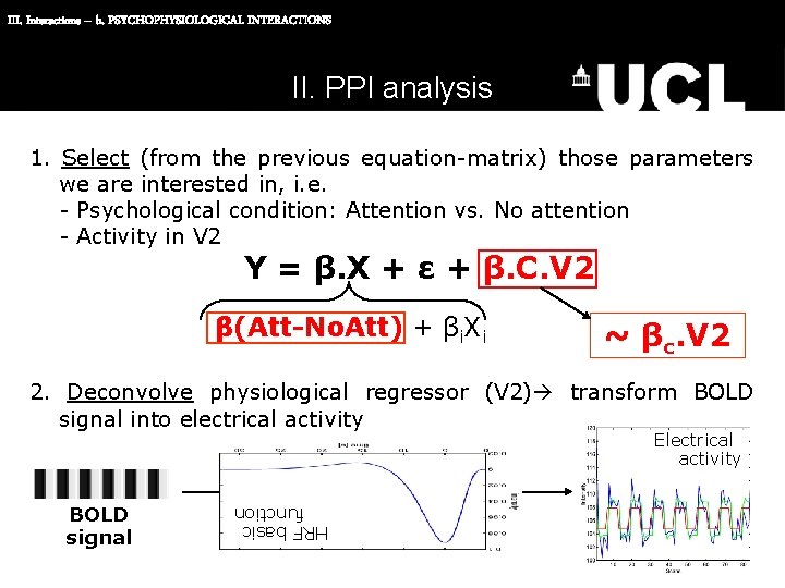
III. Interactions – b. PSYCHOPHYSIOLOGICAL INTERACTIONS Neurobiological process: Where these interactions occur? Hemodynamic vs neural level SOLUTION: 1 - Deconvolve BOLD signal corresponding to region of interest (e. g. V 2) BOLD signal in V 2 Neural activity in V 2 Psychological variable x 2 - Calculate interaction term considering neural activity psychological condition x neural activity HRF basic function 3 - Re-convolve the interaction term using HRF Gitelman et al. Neuroimage 2003

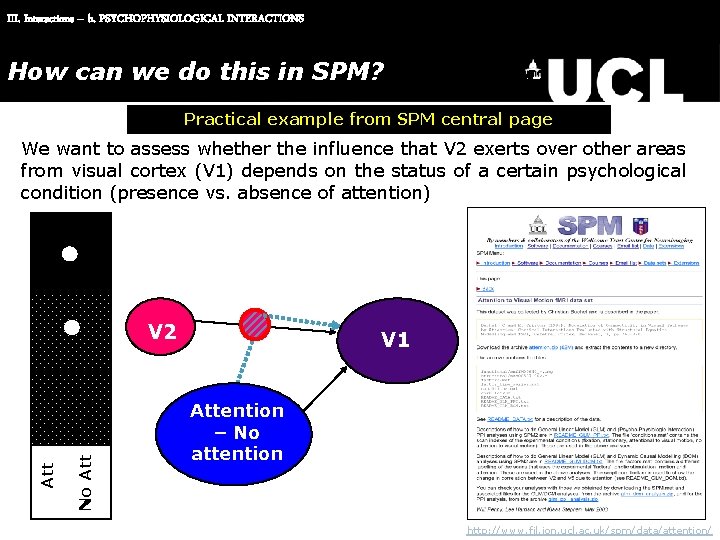
III. Interactions – b. PSYCHOPHYSIOLOGICAL INTERACTIONS How can we How do this SPM? caninwe do this in SPM? Practical example from SPM central page We want to assess whether the influence that V 2 exerts over other areas from visual cortex (V 1) depends on the status of a certain psychological condition (presence vs. absence of attention) No Att V 2 V 1 Attention – No attention http: //www. fil. ion. ucl. ac. uk/spm/data/attention/

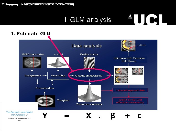
III. Interactions – b. PSYCHOPHYSIOLOGICAL INTERACTIONS I. GLM analysis 1. Estimate GLM Y = X . β + ε

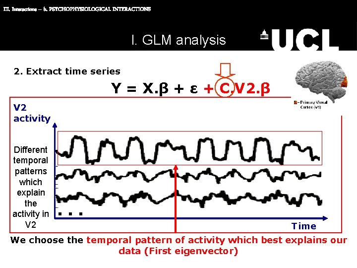
III. Interactions – b. PSYCHOPHYSIOLOGICAL INTERACTIONS I. GLM analysis 2. Extract time series Meaning? To summarise the evolution in time of the activation of a certain region Place? At region of interest (e. g. V 2) region used as explanatory variable Procedure? Principle Component Analysis (done by Singular Value Decomposition) To find those temporal patterns of activity which explain most of the variance of our region of interest these patterns are represented by the eigenvectors the variance of these eigenvectors is represented by eigenvalues Reason? To include (the most important) eigenvalues in the model we transform dynamic information into STATIC information we will work with this static information PPI is a STATIC MODEL

III. Interactions – b. PSYCHOPHYSIOLOGICAL INTERACTIONS I. GLM analysis 2. Extract time series Y = X. β + ε + C. V 2. β V 2 activity Different temporal patterns which explain the activity in V 2 … Time We choose the temporal pattern of activity which best explains our data (First eigenvector)

III. Interactions – b. PSYCHOPHYSIOLOGICAL INTERACTIONS II. PPI analysis 1. Select (from the previous equation-matrix) those parameters we are interested in, i. e. - Psychological condition: Attention vs. No attention - Activity in V 2 Y = β. X + ε + β. C. V 2 β(Att-No. Att) + βi. Xi ~ βc. V 2 2. Deconvolve physiological regressor (V 2) transform BOLD signal into electrical activity Electrical activity HRF basic function BOLD signal

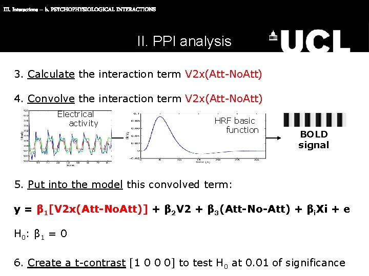
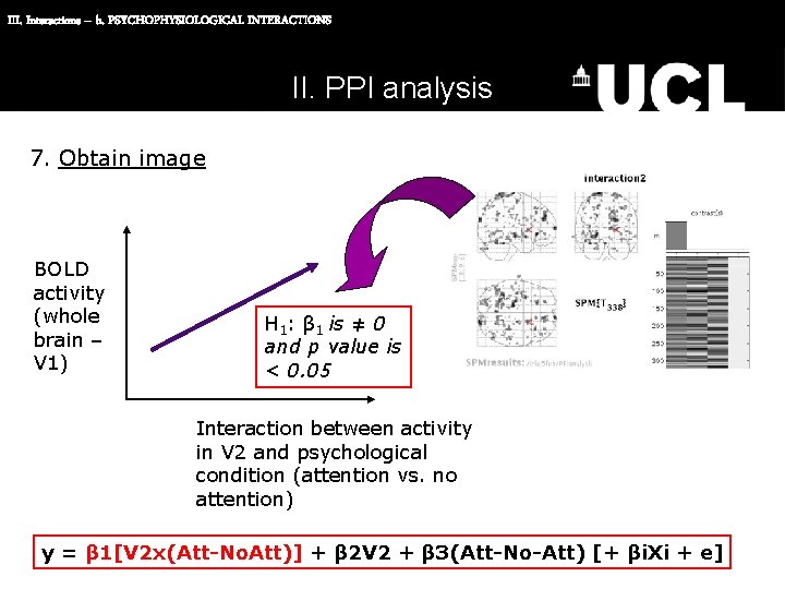
III. Interactions – b. PSYCHOPHYSIOLOGICAL INTERACTIONS II. PPI analysis 3. Calculate the interaction term V 2 x(Att-No. Att) 4. Convolve the interaction term V 2 x(Att-No. Att) Electrical activity HRF basic function BOLD signal 5. Put into the model this convolved term: y = β 1[V 2 x(Att-No. Att)] + β 2 V 2 + β 3(Att-No-Att) + βi. Xi + e H 0: β 1 = 0 6. Create a t-contrast [1 0 0 0] to test H 0 at 0. 01 of significance

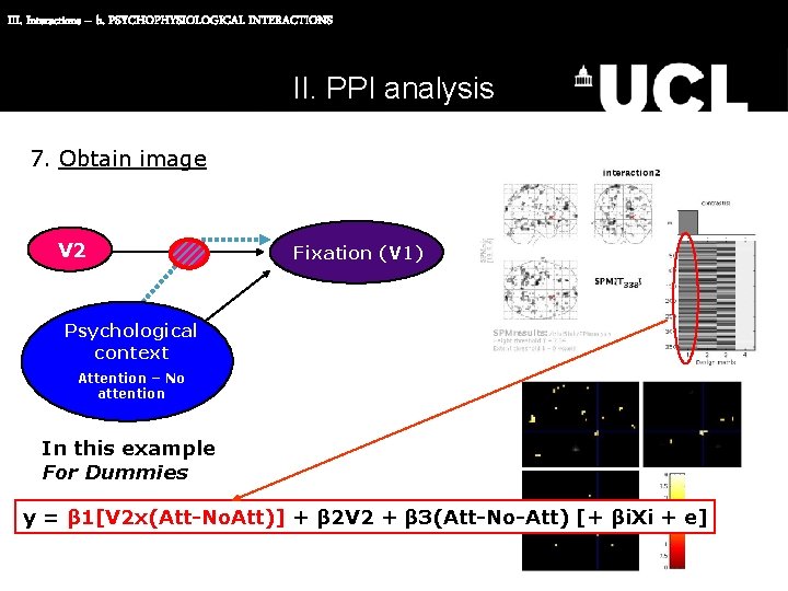
III. Interactions – b. PSYCHOPHYSIOLOGICAL INTERACTIONS II. PPI analysis 7. Obtain image V 2 Fixation (V 1) Psychological context Attention – No attention In this example For Dummies y = β 1[V 2 x(Att-No. Att)] + β 2 V 2 + β 3(Att-No-Att) [+ βi. Xi + e]

III. Interactions – b. PSYCHOPHYSIOLOGICAL INTERACTIONS II. PPI analysis 7. Obtain image BOLD activity (whole brain – V 1) H 1: β 1 is ≠ 0 and p value is < 0. 05 Interaction between activity in V 2 and psychological condition (attention vs. no attention) y = β 1[V 2 x(Att-No. Att)] + β 2 V 2 + β 3(Att-No-Att) [+ βi. Xi + e]

III. Interactions – b. PSYCHOPHYSIOLOGICAL INTERACTIONS The end (of PPI…)

Structural Equation Modelling Maria Joao Rosa, UCL, London, 24/02/2010

Introduction | Theory | Application | Limitations | Conclusions A bit of history • Since 1920 s and in economics, psychology and social sciences. • In functional imaging since early 1990 s: – Animal autoradiographic data – Human PET data (Mc. Intosh and Gonzalez-Lima, 1991) – f. MRI (Büchel and Friston, 1997)

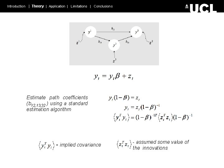
Introduction | Theory | Application | Limitations | Conclusions Definition • Structural Equation Moldelling (SEM) or ‘path analysis’: multivariate tool that is used to test hypotheses regarding the influences among interacting variables. • Neuro-SEM: – Connections between neuroanatomy. brain areas are based on known – Interregional covariances of activity are used to calculate the path coefficients representing the magnitude of the influence or directional path.

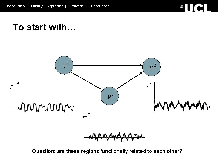
Introduction | Theory | Application | Limitations | Conclusions To start with… y 1 y 2 y 3 Question: are these regions functionally related to each other?

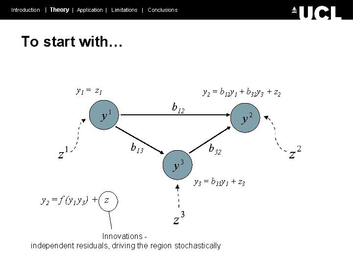
Introduction | Theory | Application | Limitations | Conclusions To start with… y 1 = z 1 y y 2 = b 12 y 1 + b 32 y 3 + z 2 b 12 1 b 13 y 2 b 32 y 3 = b 13 y 1 + z 3 y 2 = f (y 1 y 3) + z Innovations independent residuals, driving the region stochastically

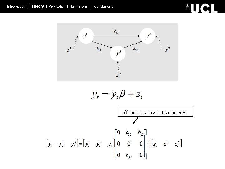
Introduction | Theory | Application | Limitations | Conclusions includes only paths of interest

Introduction | Theory | Application | Limitations | Conclusions Estimate path coefficients (b 12, 13, 32 ) using a standard estimation algorithm - implied covariance - assumed some value of the innovations

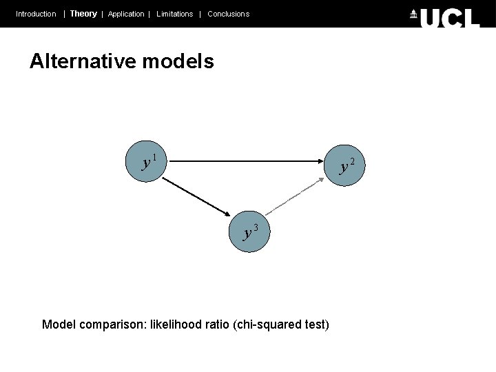
Introduction | Theory | Application | Limitations | Conclusions Alternative models y 1 y 2 y 3 Model comparison: likelihood ratio (chi-squared test)

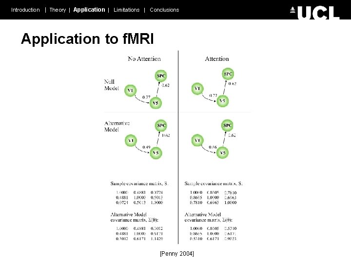
Introduction | Theory | Application | Limitations | Conclusions Application to f. MRI [Penny 2004]

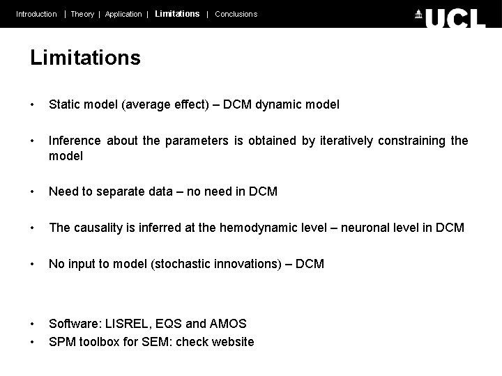
Introduction | Theory | Application | Limitations | Conclusions Limitations • Static model (average effect) – DCM dynamic model • Inference about the parameters is obtained by iteratively constraining the model • Need to separate data – no need in DCM • The causality is inferred at the hemodynamic level – neuronal level in DCM • No input to model (stochastic innovations) – DCM • • Software: LISREL, EQS and AMOS SPM toolbox for SEM: check website

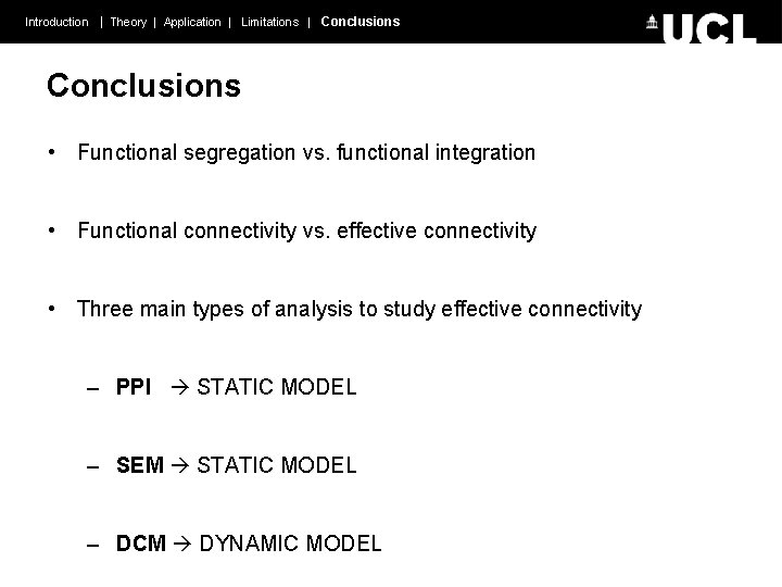
Introduction | Theory | Application | Limitations | Conclusions • Functional segregation vs. functional integration • Functional connectivity vs. effective connectivity • Three main types of analysis to study effective connectivity – PPI STATIC MODEL – SEM STATIC MODEL – DCM DYNAMIC MODEL

Further reading http: //www. fil. ion. ucl. ac. uk/mfd/page 2. html http: //en. wikibooks. org/wiki/SPM http: //www. fil. ion. ucl. ac. uk/spm/data/attention/ Friston KJ, Frith CD, Passingham RE, et al (1992). Motor practice and neuropsychological adaptation in the cerebellum: a positron tomography study. Proc R Soc Lond B (1992) 248, 223 -228. Friston KJ, Frith CD, Liddle, PF & Frackowiak, RSJ. Functional Connectivity: The principle-component analysis of large data sets, J Cereb Blood Flow & Metab (1993) 13, 5 -14 Fletcher PC, Frith CD, Grasby PM et al. Brain systems for encoding and retrieval of auditory-verbal memory. An in vivo study in humans. Brain (1995) 118, 401 -416 Friston KJ, Buechel C, Fink GR et al. Psychophysiological and Modulatory Interactions in Neuroimaging. Neuroimage (1997) 6, 218 -229 Buchel C & Friston KJ. Modulation of connectivity in visual pathways by attention: Cortical interactions evaluated with structural equation modelling & f. MRI. Cerebral Cortex (1997) 7, 768 -778 Buchel C & Friston KJ. Assessing interactions among neuronal systems using functional neuroimaging. Neural Networks (2000) 13; 871 -882. Ashburner J, Friston KJ, Penny W. Human Brain Function 2 nd EDITION (2003) Chap 18 -20 Gitelman DR, Penny WD, Ashburner J et al. Modeling regional and neuropsychologic interactions in f. MRI: The importance of hemodynamic deconvolution. Neuroimage (2003) 19; 200 -207. Slides from previous years

SPECIAL THANKS TO ANDRE MARREIROS Thanks for your attention London, February 24 th, 2010