Integer Programming q Formulations Plane scheduling Crew scheduling

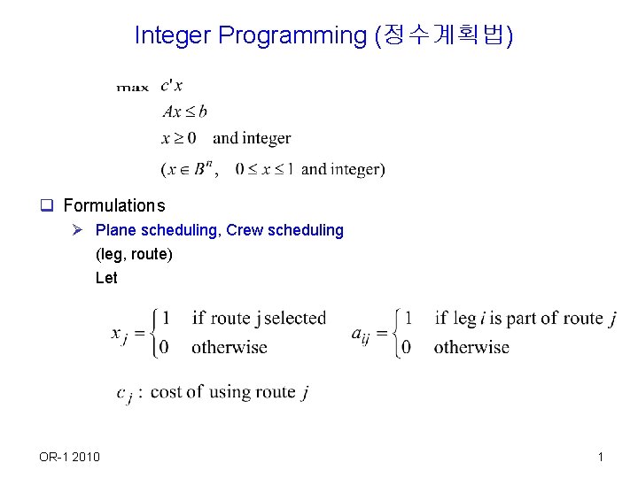
Integer Programming (정수계획법) q Formulations Ø Plane scheduling, Crew scheduling (leg, route) Let OR-1 2010 1

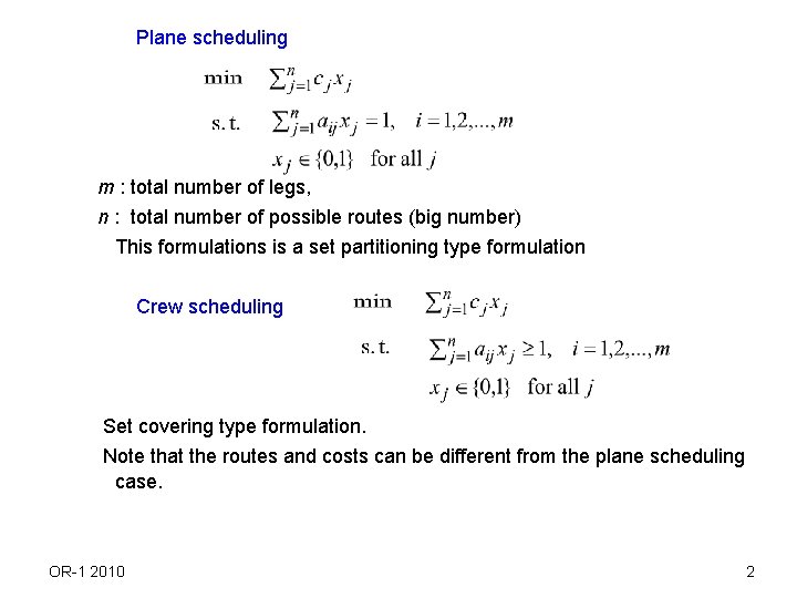
Plane scheduling m : total number of legs, n : total number of possible routes (big number) This formulations is a set partitioning type formulation Crew scheduling Set covering type formulation. Note that the routes and costs can be different from the plane scheduling case. OR-1 2010 2

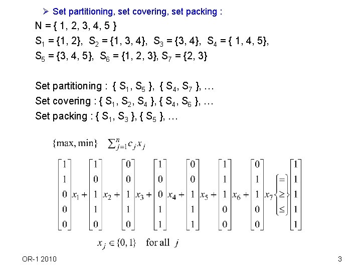
Ø Set partitioning, set covering, set packing : N = { 1, 2, 3, 4, 5 } S 1 = {1, 2}, S 2 = {1, 3, 4}, S 3 = {3, 4}, S 4 = { 1, 4, 5}, S 5 = {3, 4, 5}, S 6 = {1, 2, 3}, S 7 = {2, 3} Set partitioning : { S 1, S 5 }, { S 4, S 7 }, … Set covering : { S 1, S 2, S 4 }, { S 4, S 6 }, … Set packing : { S 1, S 3 }, { S 5 }, … OR-1 2010 3

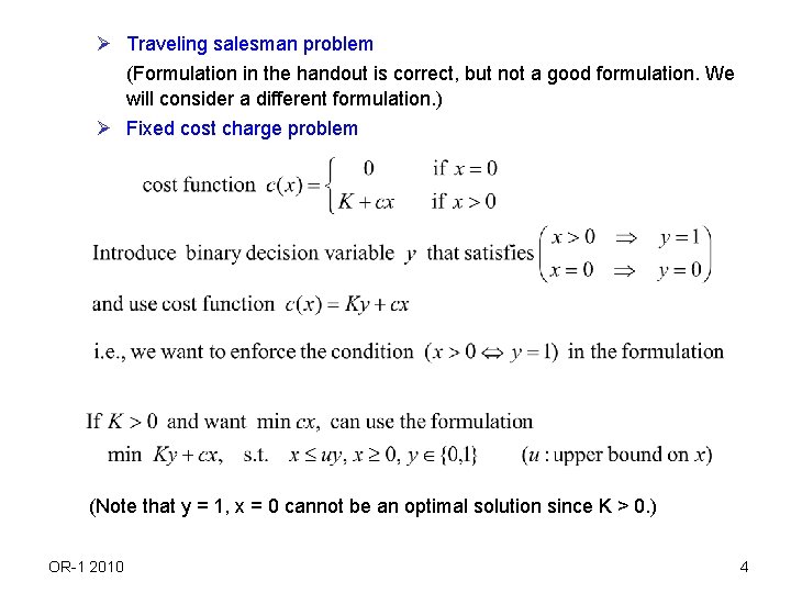
Ø Traveling salesman problem (Formulation in the handout is correct, but not a good formulation. We will consider a different formulation. ) Ø Fixed cost charge problem (Note that y = 1, x = 0 cannot be an optimal solution since K > 0. ) OR-1 2010 4

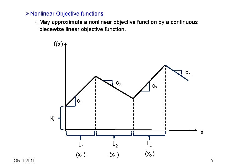
Ø Nonlinear Objective functions • May approximate a nonlinear objective function by a continuous piecewise linear objective function. f(x) c 4 c 2 c 3 c 1 K x OR-1 2010 L 1 L 2 L 3 (x 1) (x 2) (x 3) 5

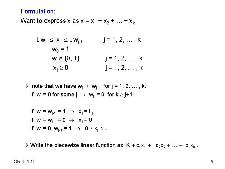
Formulation: Want to express x as x = x 1 + x 2 + … + xk Ljwj xj Ljwj-1 w 0 = 1 wj {0, 1} xj 0 j = 1, 2, … , k Ø note that we have wj wj-1 for j = 1, 2, … , k. If wj = 0 for some j wk = 0 for k j+1 If wj = wj-1 = 1 xj = Lj If wj = wj-1 = 0 xj = 0 If wj = 0, wj-1 = 1 0 xj Lj Ø Write the piecewise linear function as K + c 1 x 1 + c 2 x 2 + … + ckxk. OR-1 2010 6

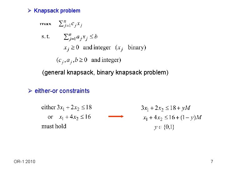
Ø Knapsack problem (general knapsack, binary knapsack problem) Ø either-or constraints OR-1 2010 7

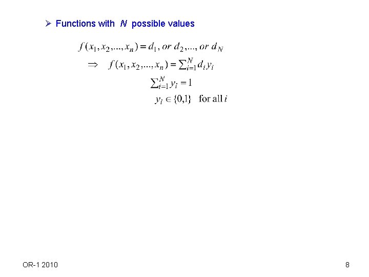
Ø Functions with N possible values OR-1 2010 8

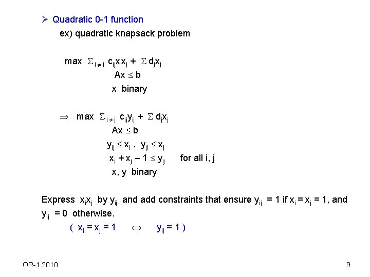
Ø Quadratic 0 -1 function ex) quadratic knapsack problem max i j cijxixj + djxj Ax b x binary max i j cijyij + djxj Ax b yij xi , yij xj xi + xj – 1 yij x, y binary for all i, j Express xixj by yij and add constraints that ensure yij = 1 if xi = xj = 1, and yij = 0 otherwise. ( xi = x j = 1 yij = 1 ) OR-1 2010 9

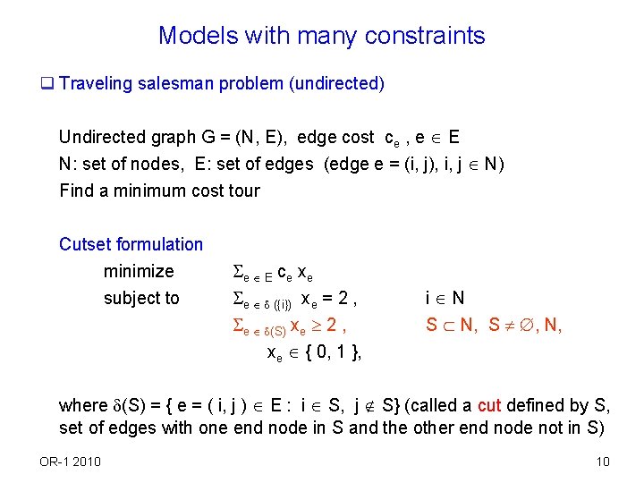
Models with many constraints q Traveling salesman problem (undirected) Undirected graph G = (N, E), edge cost ce , e E N: set of nodes, E: set of edges (edge e = (i, j), i, j N) Find a minimum cost tour Cutset formulation minimize subject to e E ce xe e ({i}) xe = 2 , e (S) xe 2 , xe { 0, 1 }, i N S N, S , N, where (S) = { e = ( i, j ) E : i S, j S} (called a cut defined by S, set of edges with one end node in S and the other end node not in S) OR-1 2010 10

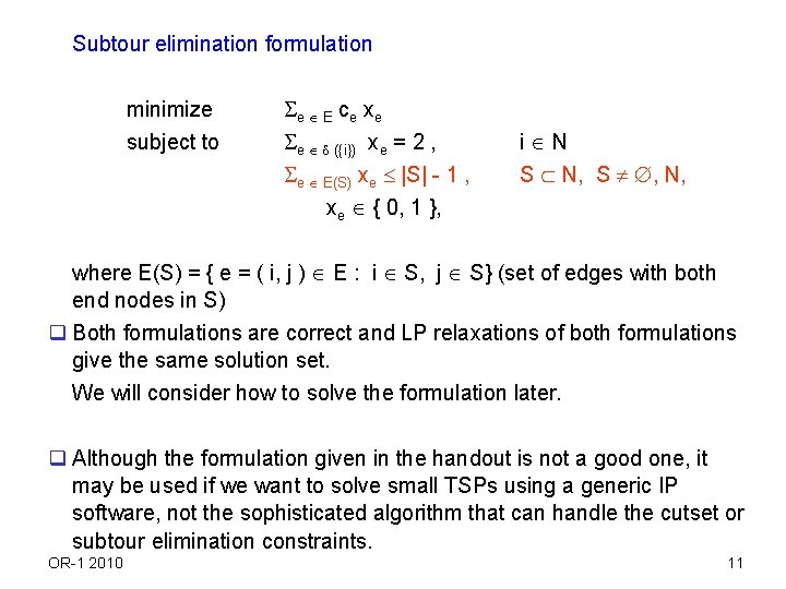
Subtour elimination formulation minimize subject to e E ce xe e ({i}) xe = 2 , e E(S) xe |S| - 1 , xe { 0, 1 }, i N S N, S , N, where E(S) = { e = ( i, j ) E : i S, j S} (set of edges with both end nodes in S) q Both formulations are correct and LP relaxations of both formulations give the same solution set. We will consider how to solve the formulation later. q Although the formulation given in the handout is not a good one, it may be used if we want to solve small TSPs using a generic IP software, not the sophisticated algorithm that can handle the cutset or subtour elimination constraints. OR-1 2010 11

q Integer programming significantly increases the modeling capability, but usually takes much more time to solve than linear programming. Theoretically, it is generally believed that there does not exist a polynomial time algorithm to solve general integer programming problems. However, recent advances in theory and software, combined with powerful computers makes it possible to solve many real world problems using integer programming. OR-1 2010 12

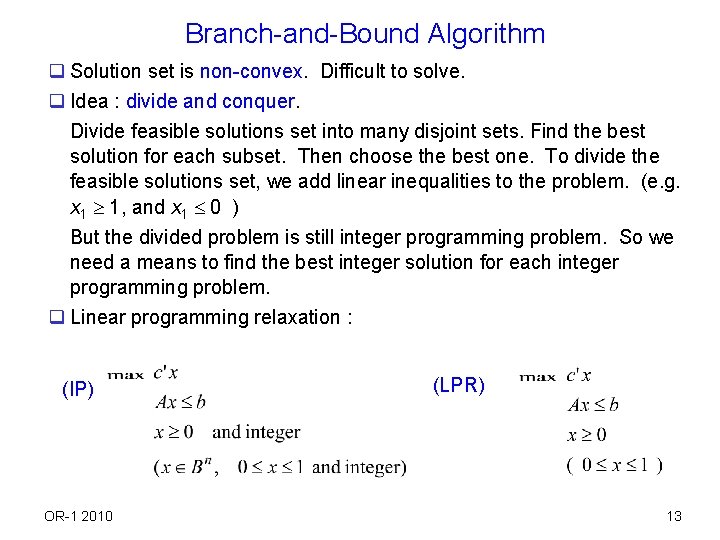
Branch-and-Bound Algorithm q Solution set is non-convex. Difficult to solve. q Idea : divide and conquer. Divide feasible solutions set into many disjoint sets. Find the best solution for each subset. Then choose the best one. To divide the feasible solutions set, we add linear inequalities to the problem. (e. g. x 1 1, and x 1 0 ) But the divided problem is still integer programming problem. So we need a means to find the best integer solution for each integer programming problem. q Linear programming relaxation : (IP) OR-1 2010 (LPR) 13

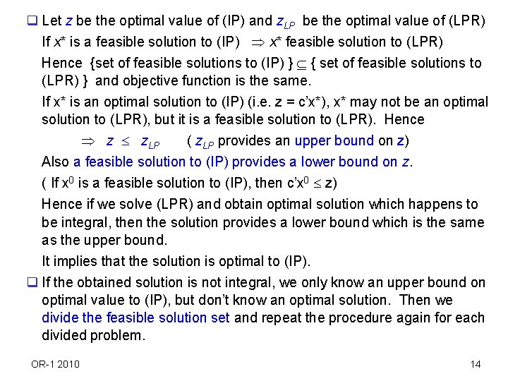
q Let z be the optimal value of (IP) and z. LP be the optimal value of (LPR) If x* is a feasible solution to (IP) x* feasible solution to (LPR) Hence {set of feasible solutions to (IP) } { set of feasible solutions to (LPR) } and objective function is the same. If x* is an optimal solution to (IP) (i. e. z = c’x*), x* may not be an optimal solution to (LPR), but it is a feasible solution to (LPR). Hence z z. LP ( z. LP provides an upper bound on z) Also a feasible solution to (IP) provides a lower bound on z. ( If x 0 is a feasible solution to (IP), then c’x 0 z) Hence if we solve (LPR) and obtain optimal solution which happens to be integral, then the solution provides a lower bound which is the same as the upper bound. It implies that the solution is optimal to (IP). q If the obtained solution is not integral, we only know an upper bound on optimal value to (IP), but don’t know an optimal solution. Then we divide the feasible solution set and repeat the procedure again for each divided problem. OR-1 2010 14

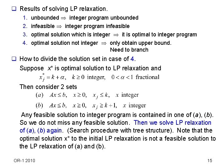
q Results of solving LP relaxation. 1. 2. 3. 4. unbounded integer program unbounded infeasible integer program infeasible optimal solution which is integer it is optimal to integer program optimal solution not integer only obtain upper bound. Need to branch q How to divide the solution set in case of 4. Suppose x* is optimal solution to LP relaxation and Then consider 2 sets Any feasible solution to integer program is contained in one of (a), (b). So we do not miss any feasible solution. Then we solve LP relaxation of (a), (b) again. (Search procedure with tree structure). Note that the optimal solution x* to the initial LP relaxation is not a feasible solution to the LP relaxation of (a) and (b). OR-1 2010 15

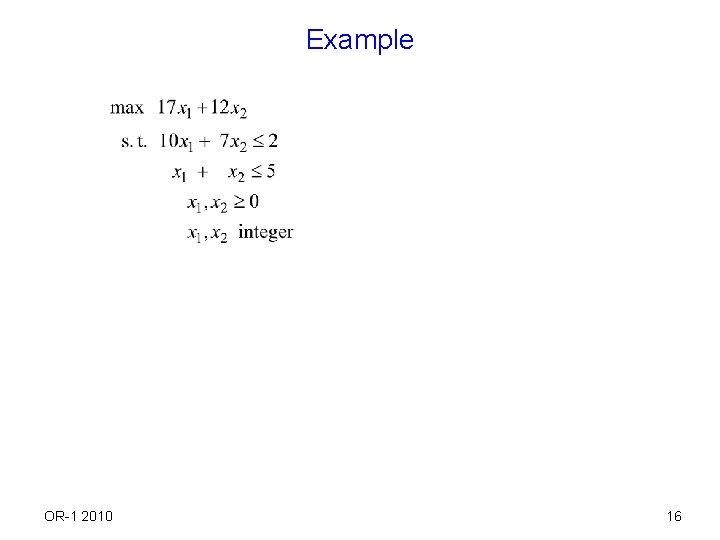
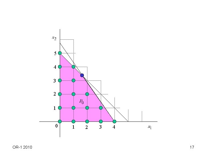
Example OR-1 2010 16

5 4 3 2 1 0 OR-1 2010 1 2 3 4 17

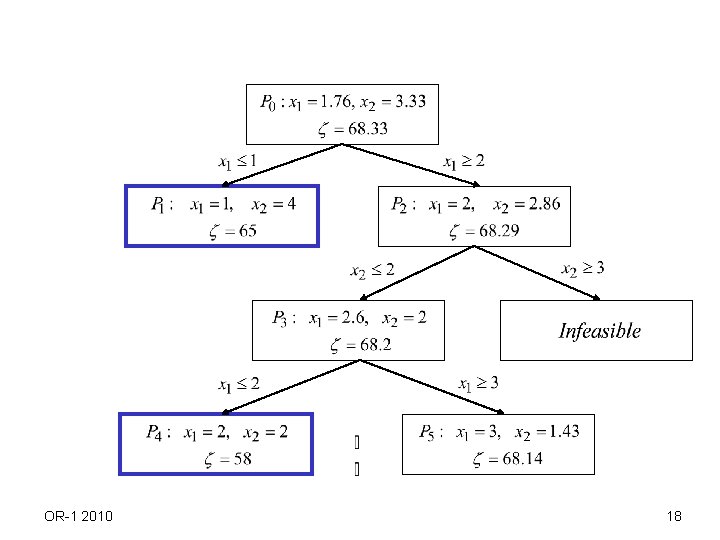
OR-1 2010 18

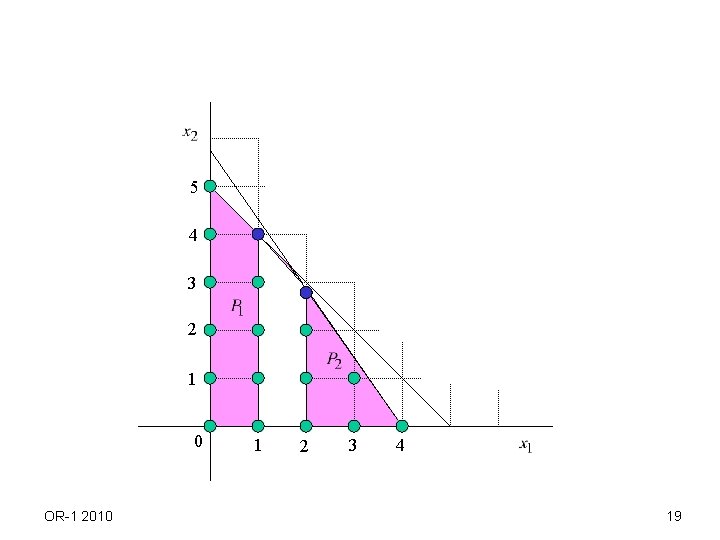
5 4 3 2 1 0 OR-1 2010 1 2 3 4 19

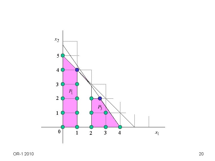
5 4 3 2 1 0 OR-1 2010 1 2 3 4 20

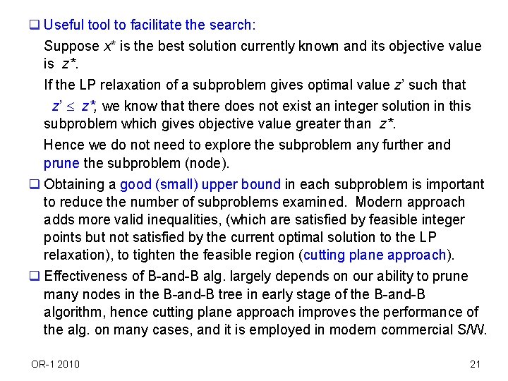
q Useful tool to facilitate the search: Suppose x* is the best solution currently known and its objective value is z*. If the LP relaxation of a subproblem gives optimal value z’ such that z’ z*, we know that there does not exist an integer solution in this subproblem which gives objective value greater than z*. Hence we do not need to explore the subproblem any further and prune the subproblem (node). q Obtaining a good (small) upper bound in each subproblem is important to reduce the number of subproblems examined. Modern approach adds more valid inequalities, (which are satisfied by feasible integer points but not satisfied by the current optimal solution to the LP relaxation), to tighten the feasible region (cutting plane approach). q Effectiveness of B-and-B alg. largely depends on our ability to prune many nodes in the B-and-B tree in early stage of the B-and-B algorithm, hence cutting plane approach improves the performance of the alg. on many cases, and it is employed in modern commercial S/W. OR-1 2010 21

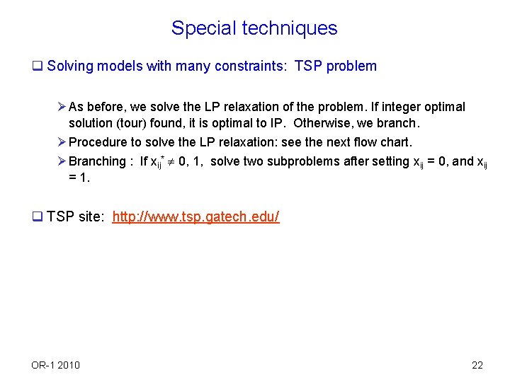
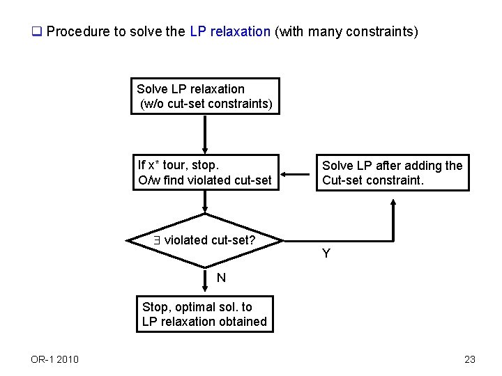
Special techniques q Solving models with many constraints: TSP problem Ø As before, we solve the LP relaxation of the problem. If integer optimal solution (tour) found, it is optimal to IP. Otherwise, we branch. Ø Procedure to solve the LP relaxation: see the next flow chart. Ø Branching : If xij* 0, 1, solve two subproblems after setting xij = 0, and xij = 1. q TSP site: http: //www. tsp. gatech. edu/ OR-1 2010 22

q Procedure to solve the LP relaxation (with many constraints) Solve LP relaxation (w/o cut-set constraints) If x* tour, stop. O/w find violated cut-set? Solve LP after adding the Cut-set constraint. Y N Stop, optimal sol. to LP relaxation obtained OR-1 2010 23

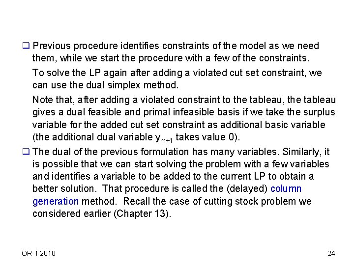
q Previous procedure identifies constraints of the model as we need them, while we start the procedure with a few of the constraints. To solve the LP again after adding a violated cut set constraint, we can use the dual simplex method. Note that, after adding a violated constraint to the tableau, the tableau gives a dual feasible and primal infeasible basis if we take the surplus variable for the added cut set constraint as additional basic variable (the additional dual variable ym+1 takes value 0). q The dual of the previous formulation has many variables. Similarly, it is possible that we can start solving the problem with a few variables and identifies a variable to be added to the current LP to obtain a better solution. That procedure is called the (delayed) column generation method. Recall the case of cutting stock problem we considered earlier (Chapter 13). OR-1 2010 24

OR-1 2010 25