Installing and Running CISMDX and Overview of Open

Installing and Running CISM_DX and Overview of Open. DX Bob Weigel The CISM Knowledge Transfer Short Course AFWA Omaha, November 2 -3, 2005

Outline • Examples – Novice User Interface • Exploring the structure of the magnetosphere • Satellite and map views of geographic model data – Advanced Analysis • Energy Partitioning in the magnetosphere – Additional Features • Coordinate system transformations • Tools for making visualizations

What is Open. DX? • An open source data visualization package based upon IBM’s commercial Data Explorer (DX) visualization system – Full featured software package for visualization scientific, engineering, and analytic data – Open system design built upon standard interface environments which allow great flexibility in creating visualizations – Very active development community Version 4. 3 available and thoroughly tested • www. opendx. org for more information

Data Structures: The Field Object • A Field is the fundamental programming object in the Open. DX • 3 main parts – Positions • Locations in space – Up to 3 D array – Connections • Explains how the positions relate to each other – Required for interpolation – Data • Actual information can be scalar, 3 -vector or beyond – Vector operations only understand Cartesian coords

Grids • The connection between points forms the grid • DX supports 3 grid types – irregular • irregular positions – irregular connections – deformed regular • irregular positions – regular connections – regular • regular positions – regular connections • Some DX modules require regular connections – e. g. slab Deformed regular Irregular Deformed regular

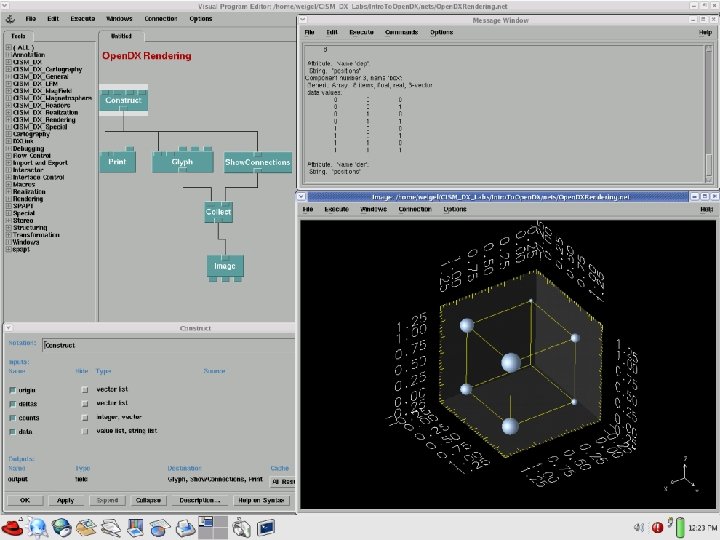
Visual Program Environment (VPE) • User ‘writes’ a visual program or net to create visualizations • These programs use the modules provided by Open. DX or modules written by the user to accomplish specific tasks such as data importing, coordinate system rotations, etc

Modules

The Map Module • The Map Module interpolates data from any DX Object to another DX Object – This includes field lines and isosurfaces – Relies on the Connections component of Open. DX Field • Velocity data from the ENLIL model is interpolated along a radial line in the ecliptic plane and displayed in a second window Thanks to Dusan Odstrcil and Nick Arge

Summer School Labs

The Compute Module • Compute module moves Open. DX from just a visualization tool into an analysis tool – Basic math, trig functions, logical, & vector operations • Works on both data and underlying grids

The. The Map Module

The Mark/Unmark modules Thanks to S. Mc. Gregor

Movie Making • Example networks and macro modules provide tools for generating movies – Easily define camera trajectory and look direction through computational domain – Sequencer and compute are used to synchronize camera motion and temporal evolution of model results Thanks to Tim Guild

Open. DX applications in CISM_DX package

LFM – Magnetospheric Model • CISM Summer School Students used this network to explore the 3 D structure of the Magnetosphere Thanks to John Lyon and Sarah Mc. Gregor

TING Visualizations • TING is a 3 D Global Circulation Model for the Earth’s Thermosphere and Ionosphere – Variables describing the action of the neutral and ion species in these domains are stored in HDF files • Networks support satellite views as well as map projections Thanks to Wenbin Wang & Tom Brecht

Coordinate Systems • SPTransform Module – utilizes the Geopack coordinate system library – allows transformation of vectors between virtually all Space Physics coordinate systems

ENLIL – Solar Wind Model • Network was used as basis for graduate student lab in CISM Summer School Thanks to Dusan Odstrcil

MAS – Coronal Results • Complicated staggered mesh required writing import module – also required transformation from Spherical to Cartesian Coordinates – Open. DX modules allowed for implementation of periodic connections in phi direction Thanks to Pete Riley and Jon Linker

LFM – L* Calculation • Electron drift trajectories are used as source points for field line tracing – End points are mapped from inner edge into ionosphere – L* is determined by calculating flux enclosed in orbit • In DX the field line is an object that can be used for interpolation Thanks to Scot Elkington

LFM – Pathlines • Streamline – Path through vector field that is tanget to vectors throughout – magnetic field lines • Pathline – Path of fluid element over a period of time – reverse time to see where elements come from • Combine pathline with streamline object to monitor flux tube volume as a function of time