Informed search algorithms Outline Generate and Test Bestfirst

Informed search algorithms

Outline • • Generate and Test Best-first search Greedy best-first search A* search Admissible Heuristic Hill-climbing search Simulated annealing search Local beam search

Generate-and-test • Very simple strategy - just keep guessing. do while goal not accomplished generate a possible solution test solution to see if it is a goal • Heuristics may be used to determine the specific rules for solution generation. 3

TSP Example A 1 2 3 5 D B 6 4 C 4

Best-First Search • Combines the advantages of Breadth-First and Depth-First searchs. – DFS: follows a single path, don’t need to generate all competing paths. – BFS: doesn’t get caught in loops or dead-endpaths. • Best First Search: explore the most promising path seen so far. 5
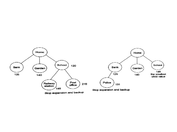
 While goal not reached: 1. Generate all potential successor states")
Best-First Search (cont. ) While goal not reached: 1. Generate all potential successor states and add to a list of states. 2. Pick the best state in the list and go to it. • Similar to steepest-ascent, but don’t throw away states that are not chosen. 6
 for each node – estimate")
Best-first search • Idea: use an evaluation function f(n) for each node – estimate of "desirability" Expand most desirable unexpanded node • Implementation: Order the nodes in fringe in decreasing order of desirability • Special cases: – greedy best-first search – A* search

Romania with step costs in km
 = h(n) (heuristic) • = estimate of")
Greedy best-first search • Evaluation function f(n) = h(n) (heuristic) • = estimate of cost from n to goal • e. g. , h. SLD(n) = straight-line distance from n to Bucharest • Greedy best-first search expands the node that appears to be closest to goal

Greedy best-first search example

Greedy best-first search example

Greedy best-first search example

Greedy best-first search example

Properties of greedy best-first search • Complete? No – can get stuck in loops, e. g. , Iasi Neamt • Time? O(bm), but a good heuristic can give dramatic improvement • Space? O(bm) -- keeps all nodes in memory • Optimal? No

A* search • Idea: avoid expanding paths that are already expensive • Evaluation function f(n) = g(n) + h(n) • g(n) = cost so far to reach n • h(n) = estimated cost from n to goal • f(n) = estimated total cost of path through n to goal

Romania with step costs in km

A* search example

A* search example

A* search example

A* search example

A* search example

A* search example
 is admissible if for every node n, h(n)")
Admissible heuristics • A heuristic h(n) is admissible if for every node n, h(n) ≤ h*(n), where h*(n) is the true cost to reach the goal state from n. • An admissible heuristic never overestimates the cost to reach the goal, i. e. , it is optimistic • Example: h. SLD(n) (never overestimates the actual road distance) • Theorem: If h(n) is admissible, A* using TREESEARCH is optimal

Underestimating Heuristic Init P R 9+1 Q 6+1 5+1 S T 6+3 5+2

Overestimating Heuristic Init P R Q 5+1 8+1 S T U 5+2 5+3 0+4 9+1

Consistent heuristics • A heuristic is consistent if for every node n, every successor n' of n generated by any action a, h(n) ≤ c(n, a, n') + h(n') • If h is consistent, we have f(n') = g(n') + h(n') = g(n) + c(n, a, n') + h(n') ≥ g(n) + h(n) = f(n) • i. e. , f(n) is non-decreasing along any path. • Theorem: If h(n) is consistent, A* using GRAPH-SEARCH is optimal

Optimality of A* • A* expands nodes in order of increasing f value • Gradually adds "f-contours" of nodes • Contour i has all nodes with f=fi, where fi < fi+1

Properties of A* • Complete? Yes (unless there are infinitely many nodes with f ≤ f(G) ) • Time? Exponential • Space? Keeps all nodes in memory • Optimal? Yes

Pros and Cons of A* • A* is optimal and optimally efficient • A* is still slow and bulky (space kills first) – Number of nodes grows exponentially with the length to goal • This is actually a function of heuristic, but they all make mistakes – A* must search all nodes within this goal contour – Finding suboptimal goals is sometimes only feasible solution – Sometimes, better heuristics are non-admissible
 = number")
Admissible heuristics E. g. , for the 8 -puzzle: • h 1(n) = number of misplaced tiles • h 2(n) = total Manhattan distance (i. e. , no. of squares from desired location of each tile) • h 1(S) = ? • h 2(S) = ?
 = number")
Admissible heuristics E. g. , for the 8 -puzzle: • h 1(n) = number of misplaced tiles • h 2(n) = total Manhattan distance (i. e. , no. of squares from desired location of each tile) • h 1(S) = ? 8 • h 2(S) = ? 3+1+2+2+2+3+3+2 = 18

Iterative Deepening A* Iterative Deepening – Remember, as in uniformed search, this was a depth-first search where the max depth was iteratively increased – As an informed search, we again perform depth-first search, but only nodes with f-cost less than or equal to smallest f-cost of nodes expanded at last iteration
 1. If cur_state=goal state Return curr_state(success!) 2. Expand(curr_node)->children 3.")
Recursive Best First Search (RBFS) 1. If cur_state=goal state Return curr_state(success!) 2. Expand(curr_node)->children 3. If empty(children) return failure 4. Do For each c(child of the curr_node) f[c]=maximum(g(c)+h(c), f[curr_node]) Best cost=lowest of f-cost, i. e. , f[c] If(best cost>prev f-cost found) return failure Consider the alternative f-cost Goto to step 1 with (best-cost node, min(f-cost, alternative f-cost)

Disadvantage of RBFS • Generation of same states again and again. • Memory utilisation is just f-cost.

Hill-climbing search • "Like climbing Everest in thick fog with amnesia"

Hill-climbing search • Problem: depending on initial state, can get stuck in local maxima

Steepest-Ascent Hill Climbing • A variation on simple hill climbing. • Instead of moving to the first state that is better, move to the best possible state that is one move away. • The order of operators does not matter. • Not just climbing to a better state, climbing up the steepest slope. 38

Hill Climbing Termination • Local Optimum: all neighboring states are worse or the same. • Plateau - all neighboring states are the same as the current state. • Ridge - local optimum that is caused by inability to apply 2 operators at once. 39

Simulated annealing search • Idea: escape local maxima by allowing some "bad" moves but gradually decrease their frequency

Simulated annealing search

Properties of simulated annealing search • One can prove: If T decreases slowly enough, then simulated annealing search will find a global optimum with probability approaching 1 • Widely used in VLSI layout, airline scheduling, etc

Local beam search • Keep track of k states rather than just one • Start with k randomly generated states • At each iteration, all the successors of all k states are generated • If any one is a goal state, stop; else select the k best successors from the complete list and repeat.

Local Beam Search

Tabu Search

A Tabu search can have stopping criteria like a number of solutions to be explored or the neighbourhood is empty • Pros: 1. It allows to exit from sub-optimal regions by making non-improving solution to be accepted. 2. The use of tabu list improves efficiency. 3. It can be applied to both discrete and continuous solution spaces. 4. It can address difficult problems. Tabu search obtains solutions that often surpass the best solutions previously found by the other approaches. • Cons: 1. It has higher dimensions and parameters. 2. Number of iterations could be very large 3. It cannot find global optimum in some cases.
- Slides: 46