Artificial intelligence informed search AI 1 Outline Informed

Artificial intelligence: informed search AI 1

Outline Informed = use problem-specific knowledge Which search strategies? – Best-first search and its variants Heuristic functions? – How to invent them Local search and optimization – Hill climbing, local beam search, genetic algorithms, … Local search in continuous spaces Online search agents AI 1 4 -3 -2021 Pag. 2

Previously: tree-search function TREE-SEARCH(problem, fringe) return a solution or failure fringe INSERT(MAKE-NODE(INITIAL-STATE[problem]), fringe) loop do if EMPTY? (fringe) then return failure node REMOVE-FIRST(fringe) if GOAL-TEST[problem] applied to STATE[node] succeeds then return SOLUTION(node) fringe INSERT-ALL(EXPAND(node, problem), fringe) A strategy is defined by picking the order of node expansion AI 1 4 -3 -2021 Pag. 3

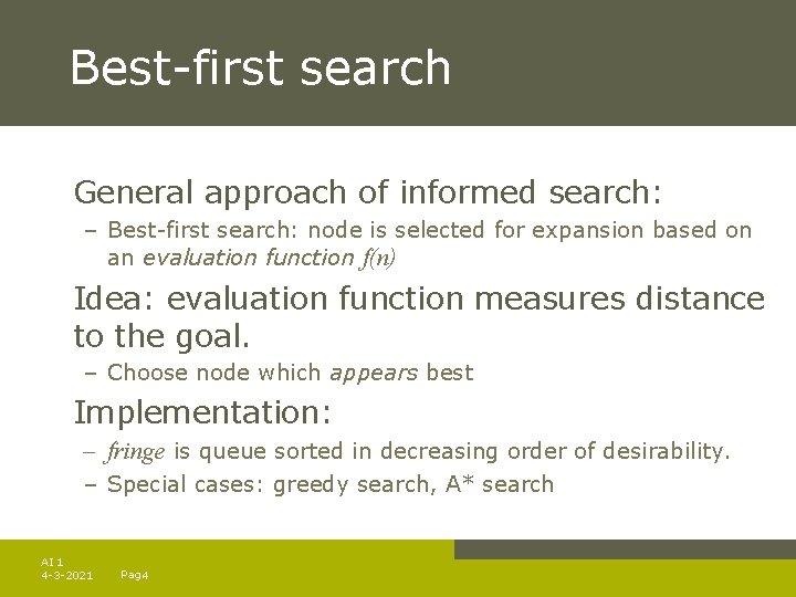
Best-first search General approach of informed search: – Best-first search: node is selected for expansion based on an evaluation function f(n) Idea: evaluation function measures distance to the goal. – Choose node which appears best Implementation: – fringe is queue sorted in decreasing order of desirability. – Special cases: greedy search, A* search AI 1 4 -3 -2021 Pag. 4

A heuristic function [dictionary]“A rule of thumb, simplification, or educated guess that reduces or limits the search for solutions in domains that are difficult and poorly understood. ” – h(n) = estimated cost of the cheapest path from node n to goal node. – If n is goal then h(n)=0 More information later. AI 1 4 -3 -2021 Pag. 5

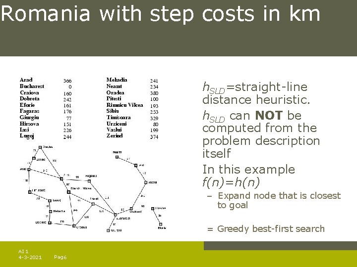
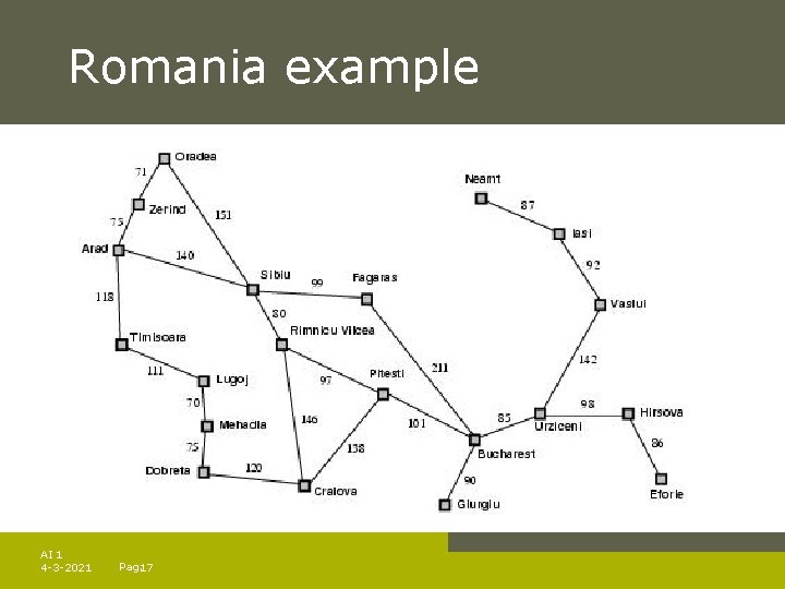
Romania with step costs in km h. SLD=straight-line distance heuristic. h. SLD can NOT be computed from the problem description itself In this example f(n)=h(n) – Expand node that is closest to goal = Greedy best-first search AI 1 4 -3 -2021 Pag. 6

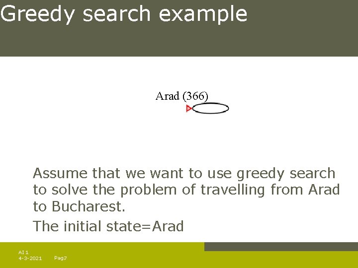
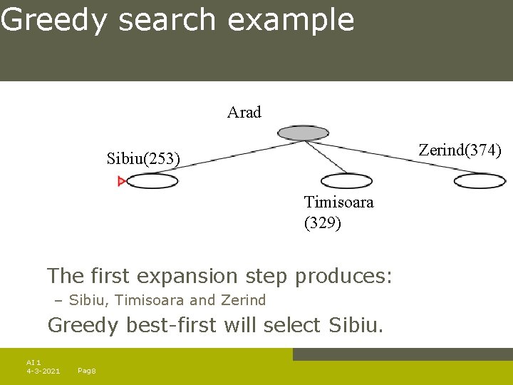
Greedy search example Arad (366) Assume that we want to use greedy search to solve the problem of travelling from Arad to Bucharest. The initial state=Arad AI 1 4 -3 -2021 Pag. 7

Greedy search example Arad Zerind(374) Sibiu(253) Timisoara (329) The first expansion step produces: – Sibiu, Timisoara and Zerind Greedy best-first will select Sibiu. AI 1 4 -3 -2021 Pag. 8

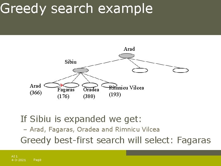
Greedy search example Arad Sibiu Arad (366) Fagaras (176) Oradea (380) Rimnicu Vilcea (193) If Sibiu is expanded we get: – Arad, Fagaras, Oradea and Rimnicu Vilcea Greedy best-first search will select: Fagaras AI 1 4 -3 -2021 Pag. 9

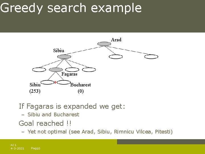
Greedy search example Arad Sibiu Fagaras Sibiu (253) Bucharest (0) If Fagaras is expanded we get: – Sibiu and Bucharest Goal reached !! – Yet not optimal (see Arad, Sibiu, Rimnicu Vilcea, Pitesti) AI 1 4 -3 -2021 Pag. 10

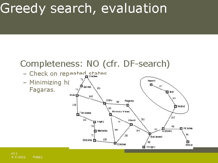
Greedy search, evaluation Completeness: NO (cfr. DF-search) – Check on repeated states – Minimizing h(n) can result in false starts, e. g. Iasi to Fagaras. AI 1 4 -3 -2021 Pag. 11

Greedy search, evaluation Completeness: NO (cfr. DF-search) Time complexity? – Cfr. Worst-case DF-search (with m is maximum depth of search space) – Good heuristic can give dramatic improvement. AI 1 4 -3 -2021 Pag. 12

Greedy search, evaluation Completeness: NO (cfr. DF-search) Time complexity: Space complexity: – Keeps all nodes in memory AI 1 4 -3 -2021 Pag. 13

Greedy search, evaluation Completeness: NO (cfr. DF-search) Time complexity: Space complexity: Optimality? NO – Same as DF-search AI 1 4 -3 -2021 Pag. 14

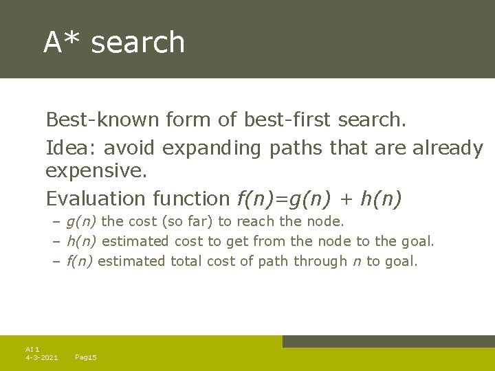
A* search Best-known form of best-first search. Idea: avoid expanding paths that are already expensive. Evaluation function f(n)=g(n) + h(n) – g(n) the cost (so far) to reach the node. – h(n) estimated cost to get from the node to the goal. – f(n) estimated total cost of path through n to goal. AI 1 4 -3 -2021 Pag. 15

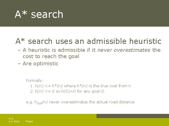
A* search uses an admissible heuristic – A heuristic is admissible if it never overestimates the cost to reach the goal – Are optimistic Formally: 1. h(n) <= h*(n) where h*(n) is the true cost from n 2. h(n) >= 0 so h(G)=0 for any goal G. e. g. h. SLD(n) never overestimates the actual road distance AI 1 4 -3 -2021 Pag. 16

Romania example AI 1 4 -3 -2021 Pag. 17

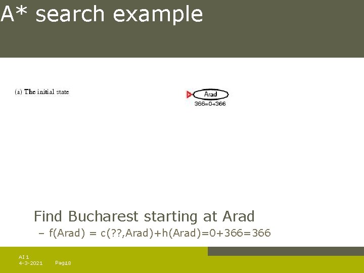
A* search example Find Bucharest starting at Arad – f(Arad) = c(? ? , Arad)+h(Arad)=0+366=366 AI 1 4 -3 -2021 Pag. 18

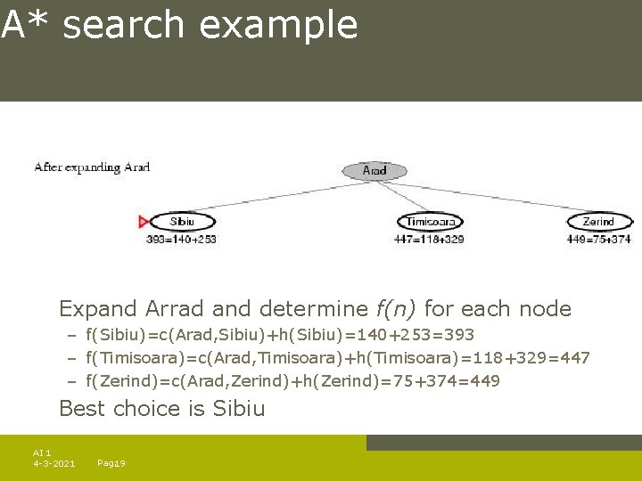
A* search example Expand Arrad and determine f(n) for each node – f(Sibiu)=c(Arad, Sibiu)+h(Sibiu)=140+253=393 – f(Timisoara)=c(Arad, Timisoara)+h(Timisoara)=118+329=447 – f(Zerind)=c(Arad, Zerind)+h(Zerind)=75+374=449 Best choice is Sibiu AI 1 4 -3 -2021 Pag. 19

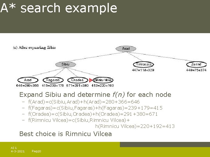
A* search example Expand Sibiu and determine f(n) for each node – – f(Arad)=c(Sibiu, Arad)+h(Arad)=280+366=646 f(Fagaras)=c(Sibiu, Fagaras)+h(Fagaras)=239+179=415 f(Oradea)=c(Sibiu, Oradea)+h(Oradea)=291+380=671 f(Rimnicu Vilcea)=c(Sibiu, Rimnicu Vilcea)+ h(Rimnicu Vilcea)=220+192=413 Best choice is Rimnicu Vilcea AI 1 4 -3 -2021 Pag. 20

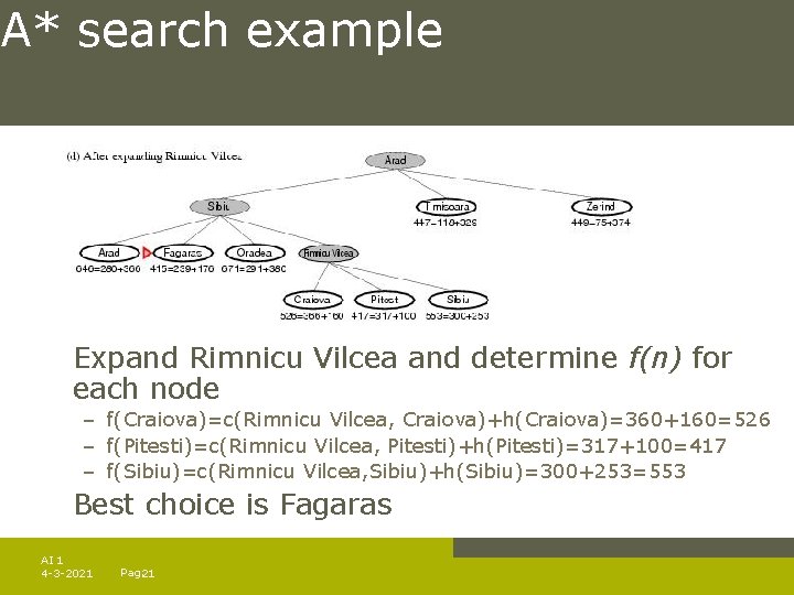
A* search example Expand Rimnicu Vilcea and determine f(n) for each node – f(Craiova)=c(Rimnicu Vilcea, Craiova)+h(Craiova)=360+160=526 – f(Pitesti)=c(Rimnicu Vilcea, Pitesti)+h(Pitesti)=317+100=417 – f(Sibiu)=c(Rimnicu Vilcea, Sibiu)+h(Sibiu)=300+253=553 Best choice is Fagaras AI 1 4 -3 -2021 Pag. 21

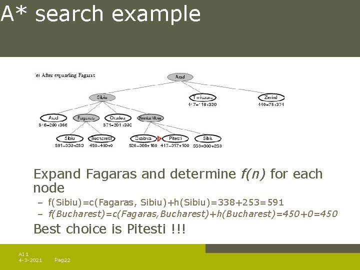
A* search example Expand Fagaras and determine f(n) for each node – f(Sibiu)=c(Fagaras, Sibiu)+h(Sibiu)=338+253=591 – f(Bucharest)=c(Fagaras, Bucharest)+h(Bucharest)=450+0=450 Best choice is Pitesti !!! AI 1 4 -3 -2021 Pag. 22

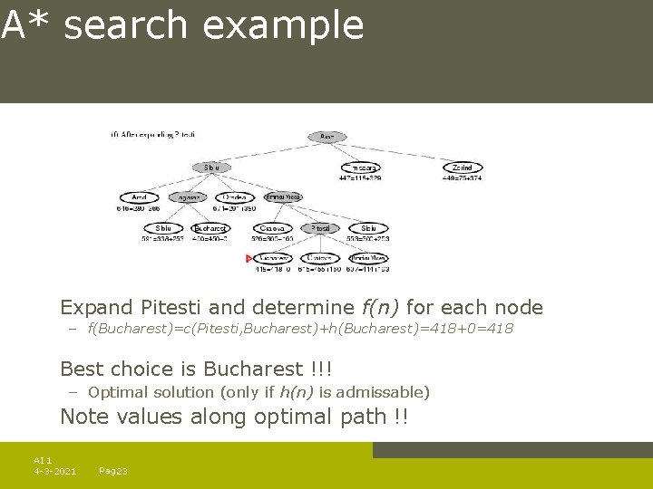
A* search example Expand Pitesti and determine f(n) for each node – f(Bucharest)=c(Pitesti, Bucharest)+h(Bucharest)=418+0=418 Best choice is Bucharest !!! – Optimal solution (only if h(n) is admissable) Note values along optimal path !! AI 1 4 -3 -2021 Pag. 23

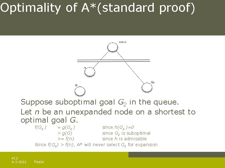
Optimality of A*(standard proof) Suppose suboptimal goal G 2 in the queue. Let n be an unexpanded node on a shortest to optimal goal G. f(G 2 ) = g(G 2 ) since h(G 2 )=0 > g(G) since G 2 is suboptimal >= f(n) since h is admissible Since f(G 2) > f(n), A* will never select G 2 for expansion AI 1 4 -3 -2021 Pag. 24

BUT … graph search Discards new paths to repeated state. – Previous proof breaks down Solution: – Add extra bookkeeping i. e. remove more expsive of two paths. – Ensure that optimal path to any repeated state is always first followed. – Extra requirement on h(n): consistency (monotonicity) AI 1 4 -3 -2021 Pag. 25

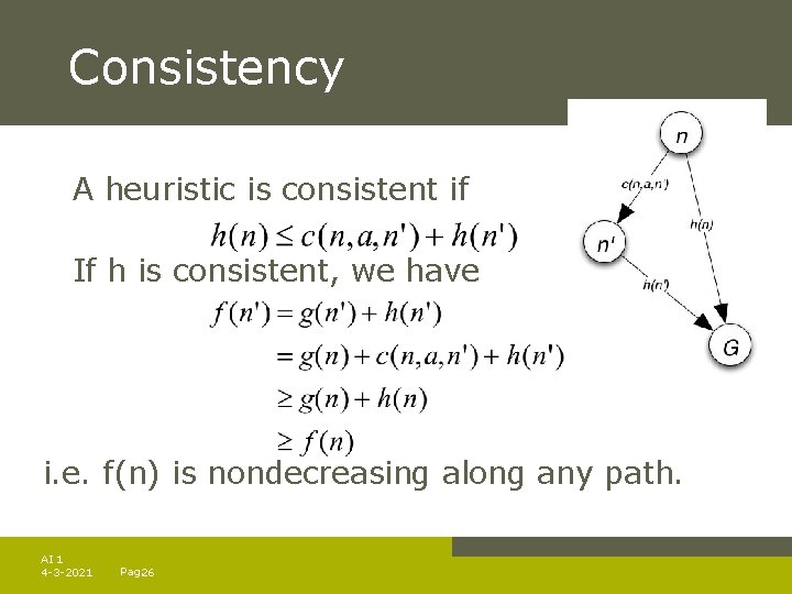
Consistency A heuristic is consistent if If h is consistent, we have i. e. f(n) is nondecreasing along any path. AI 1 4 -3 -2021 Pag. 26

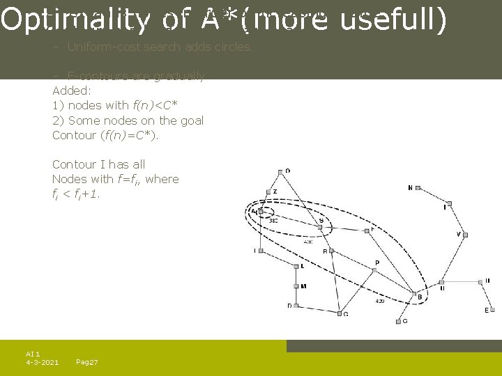
Optimality of A*(more usefull) A* expands nodes in order of increasing f value Contours can be drawn in state space – Uniform-cost search adds circles. – F-contours are gradually Added: 1) nodes with f(n)<C* 2) Some nodes on the goal Contour (f(n)=C*). Contour I has all Nodes with f=fi, where fi < fi+1. AI 1 4 -3 -2021 Pag. 27

A* search, evaluation Completeness: YES – Since bands of increasing f are added – Unless there are infinitly many nodes with f<f(G) AI 1 4 -3 -2021 Pag. 28

A* search, evaluation Completeness: YES Time complexity: – Number of nodes expanded is still exponential in the length of the solution. AI 1 4 -3 -2021 Pag. 29

A* search, evaluation Completeness: YES Time complexity: (exponential with path length) Space complexity: – It keeps all generated nodes in memory – Hence space is the major problem not time AI 1 4 -3 -2021 Pag. 30

A* search, evaluation Completeness: YES Time complexity: (exponential with path length) Space complexity: (all nodes are stored) Optimality: YES – – Cannot expand fi+1 until fi is finished. A* expands all nodes with f(n)< C* A* expands some nodes with f(n)=C* A* expands no nodes with f(n)>C* Also optimally efficient (not including ties) AI 1 4 -3 -2021 Pag. 31

Memory-bounded heuristic search Some solutions to A* space problems (maintain completeness and optimality) – Iterative-deepening A* (IDA*) – Here cutoff information is the f-cost (g+h) instead of depth – Recursive best-first search(RBFS) – Recursive algorithm that attempts to mimic standard best-first search with linear space. – (simple) Memory-bounded A* ((S)MA*) – Drop the worst-leaf node when memory is full AI 1 4 -3 -2021 Pag. 32

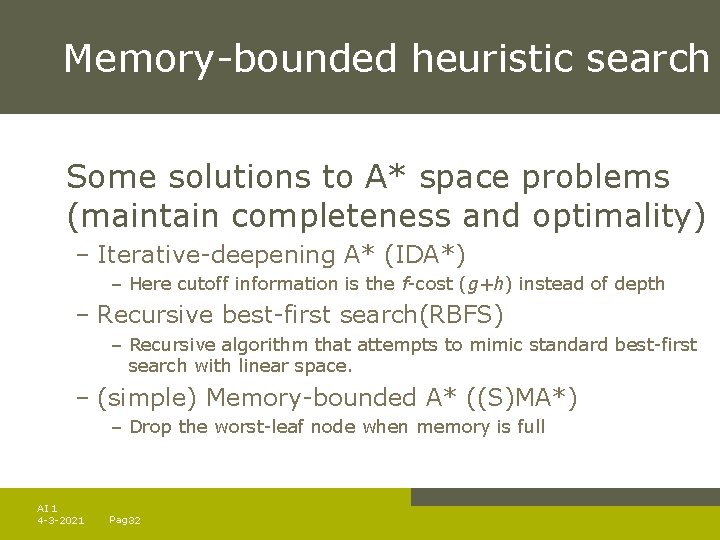
Recursive best-first search function RECURSIVE-BEST-FIRST-SEARCH(problem) return a solution or failure return RFBS(problem, MAKE-NODE(INITIAL-STATE[problem]), ∞) function RFBS( problem, node, f_limit) return a solution or failure and a new fcost limit if GOAL-TEST[problem](STATE[node]) then return node successors EXPAND(node, problem) if successors is empty then return failure, ∞ for each s in successors do f [s] max(g(s) + h(s), f [node]) repeat best the lowest f-value node in successors if f [best] > f_limit then return failure, f [best] alternative the second lowest f-value among successors result, f [best] RBFS(problem, best, min(f_limit, alternative)) if result failure then return result AI 1 4 -3 -2021 Pag. 33

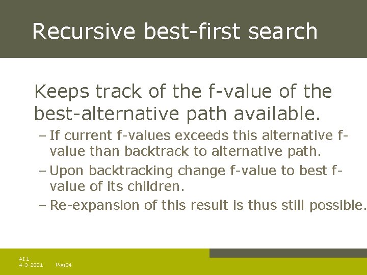
Recursive best-first search Keeps track of the f-value of the best-alternative path available. – If current f-values exceeds this alternative fvalue than backtrack to alternative path. – Upon backtracking change f-value to best fvalue of its children. – Re-expansion of this result is thus still possible. AI 1 4 -3 -2021 Pag. 34

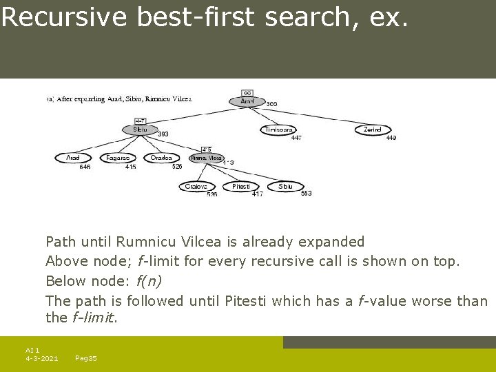
Recursive best-first search, ex. Path until Rumnicu Vilcea is already expanded Above node; f-limit for every recursive call is shown on top. Below node: f(n) The path is followed until Pitesti which has a f-value worse than the f-limit. AI 1 4 -3 -2021 Pag. 35

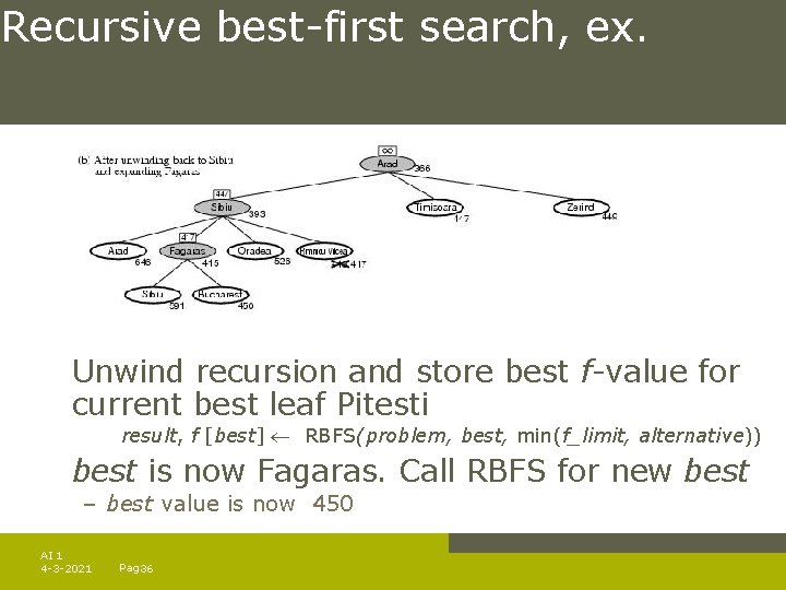
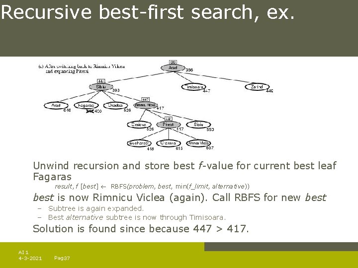
Recursive best-first search, ex. Unwind recursion and store best f-value for current best leaf Pitesti result, f [best] RBFS(problem, best, min(f_limit, alternative)) best is now Fagaras. Call RBFS for new best – best value is now 450 AI 1 4 -3 -2021 Pag. 36

Recursive best-first search, ex. Unwind recursion and store best f-value for current best leaf Fagaras result, f [best] RBFS(problem, best, min(f_limit, alternative)) best is now Rimnicu Viclea (again). Call RBFS for new best – Subtree is again expanded. – Best alternative subtree is now through Timisoara. Solution is found since because 447 > 417. AI 1 4 -3 -2021 Pag. 37

RBFS evaluation RBFS is a bit more efficient than IDA* – Still excessive node generation (mind changes) Like A*, optimal if h(n) is admissible Space complexity is O(bd). – IDA* retains only one single number (the current f-cost limit) Time complexity difficult to characterize – Depends on accuracy if h(n) and how often best path changes. IDA* en RBFS suffer from too little memory. AI 1 4 -3 -2021 Pag. 38

(simplified) memory-bounded A* Use all available memory. – I. e. expand best leafs until available memory is full – When full, SMA* drops worst leaf node (highest f-value) – Like RFBS backup forgotten node to its parent What if all leafs have the same f-value? – Same node could be selected for expansion and deletion. – SMA* solves this by expanding newest best leaf and deleting oldest worst leaf. SMA* is complete if solution is reachable, optimal if optimal solution is reachable. AI 1 4 -3 -2021 Pag. 39

Learning to search better All previous algorithms use fixed strategies. Agents can learn to improve their search by exploiting the meta-level state space. – Each meta-level state is a internal (computational) state of a program that is searching in the object-level state space. – In A* such a state consists of the current search tree A meta-level learning algorithm from experiences at the meta-level. AI 1 4 -3 -2021 Pag. 40

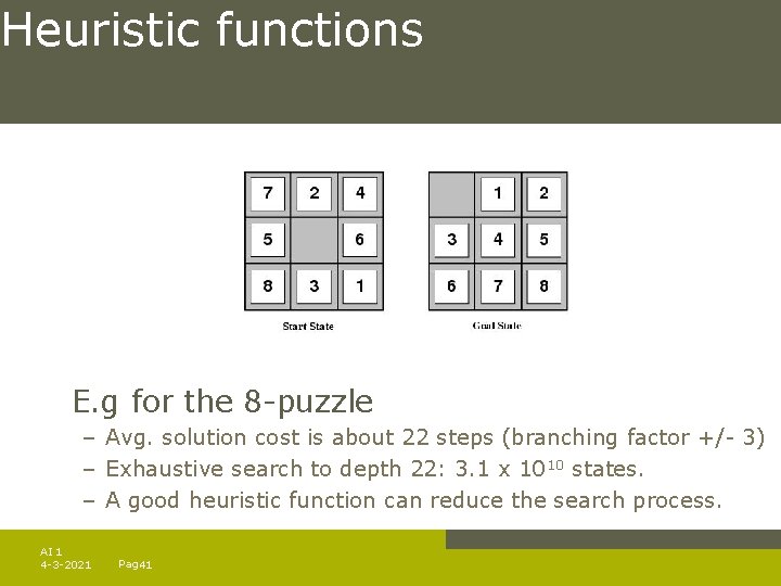
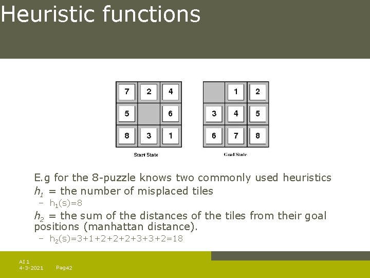
Heuristic functions E. g for the 8 -puzzle – Avg. solution cost is about 22 steps (branching factor +/- 3) – Exhaustive search to depth 22: 3. 1 x 1010 states. – A good heuristic function can reduce the search process. AI 1 4 -3 -2021 Pag. 41

Heuristic functions E. g for the 8 -puzzle knows two commonly used heuristics h 1 = the number of misplaced tiles – h 1(s)=8 h 2 = the sum of the distances of the tiles from their goal positions (manhattan distance). – h 2(s)=3+1+2+2+2+3+3+2=18 AI 1 4 -3 -2021 Pag. 42

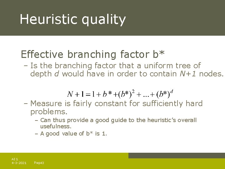
Heuristic quality Effective branching factor b* – Is the branching factor that a uniform tree of depth d would have in order to contain N+1 nodes. – Measure is fairly constant for sufficiently hard problems. – Can thus provide a good guide to the heuristic’s overall usefulness. – A good value of b* is 1. AI 1 4 -3 -2021 Pag. 43

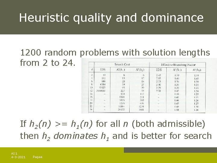
Heuristic quality and dominance 1200 random problems with solution lengths from 2 to 24. If h 2(n) >= h 1(n) for all n (both admissible) then h 2 dominates h 1 and is better for search AI 1 4 -3 -2021 Pag. 44

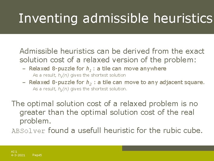
Inventing admissible heuristics Admissible heuristics can be derived from the exact solution cost of a relaxed version of the problem: – Relaxed 8 -puzzle for h 1 : a tile can move anywhere As a result, h 1(n) gives the shortest solution – Relaxed 8 -puzzle for h 2 : a tile can move to any adjacent square. As a result, h 2(n) gives the shortest solution. The optimal solution cost of a relaxed problem is no greater than the optimal solution cost of the real problem. ABSolver found a usefull heuristic for the rubic cube. AI 1 4 -3 -2021 Pag. 45

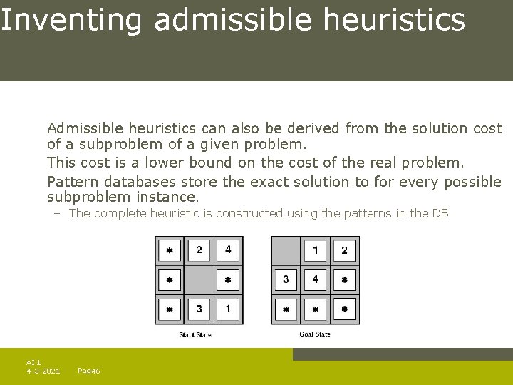
Inventing admissible heuristics Admissible heuristics can also be derived from the solution cost of a subproblem of a given problem. This cost is a lower bound on the cost of the real problem. Pattern databases store the exact solution to for every possible subproblem instance. – The complete heuristic is constructed using the patterns in the DB AI 1 4 -3 -2021 Pag. 46

Inventing admissible heuristics Another way to find an admissible heuristic is through learning from experience: – Experience = solving lots of 8 -puzzles – An inductive learning algorithm can be used to predict costs for other states that arise during search. AI 1 4 -3 -2021 Pag. 47

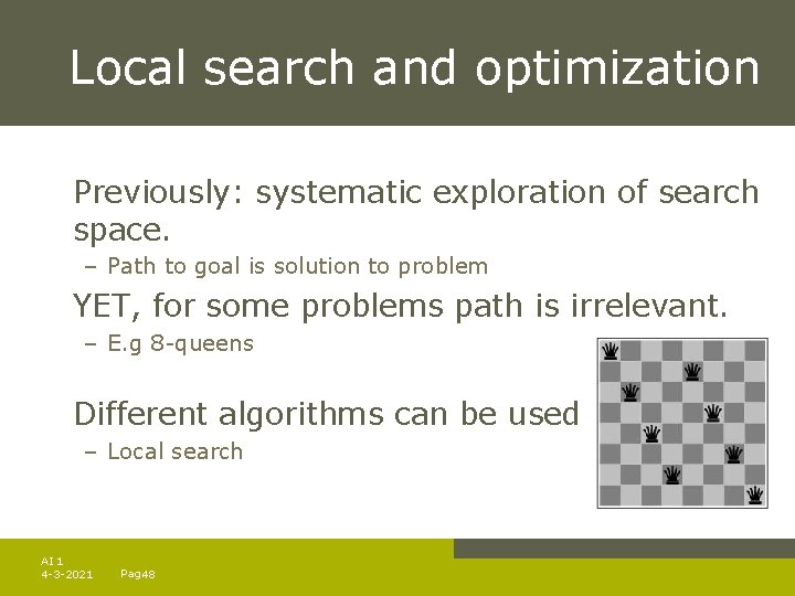
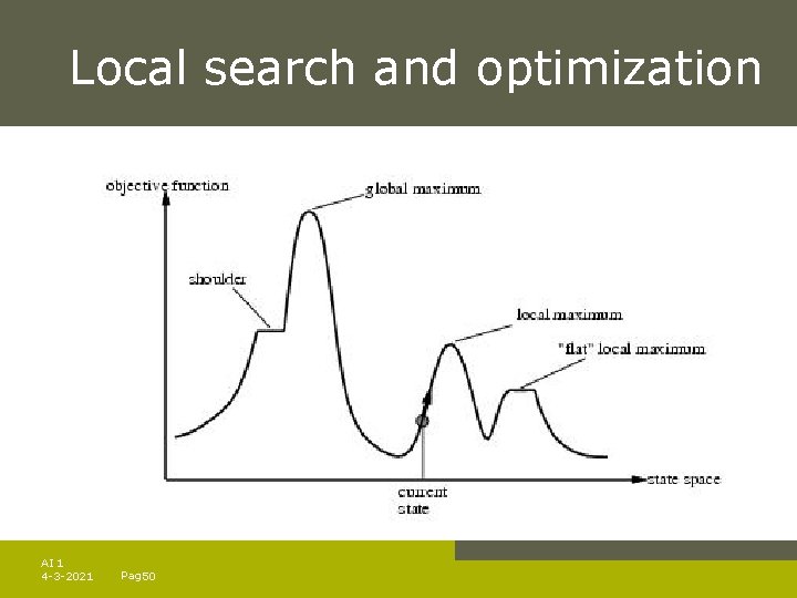
Local search and optimization Previously: systematic exploration of search space. – Path to goal is solution to problem YET, for some problems path is irrelevant. – E. g 8 -queens Different algorithms can be used – Local search AI 1 4 -3 -2021 Pag. 48

Local search and optimization Local search= use single current state and move to neighboring states. Advantages: – Use very little memory – Find often reasonable solutions in large or infinite state spaces. Are also useful for pure optimization problems. – Find best state according to some objective function. – e. g. survival of the fittest as a metaphor for optimization. AI 1 4 -3 -2021 Pag. 49

Local search and optimization AI 1 4 -3 -2021 Pag. 50

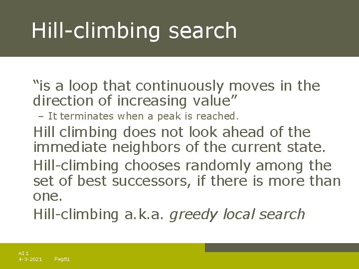
Hill-climbing search “is a loop that continuously moves in the direction of increasing value” – It terminates when a peak is reached. Hill climbing does not look ahead of the immediate neighbors of the current state. Hill-climbing chooses randomly among the set of best successors, if there is more than one. Hill-climbing a. k. a. greedy local search AI 1 4 -3 -2021 Pag. 51

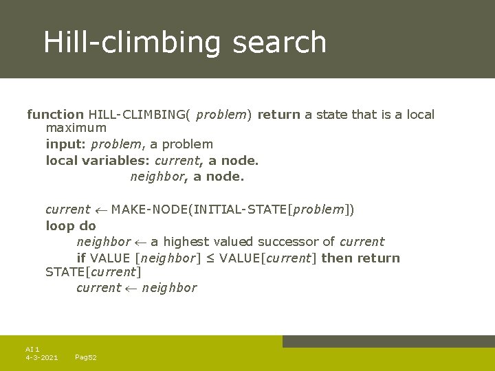
Hill-climbing search function HILL-CLIMBING( problem) return a state that is a local maximum input: problem, a problem local variables: current, a node. neighbor, a node. current MAKE-NODE(INITIAL-STATE[problem]) loop do neighbor a highest valued successor of current if VALUE [neighbor] ≤ VALUE[current] then return STATE[current] current neighbor AI 1 4 -3 -2021 Pag. 52

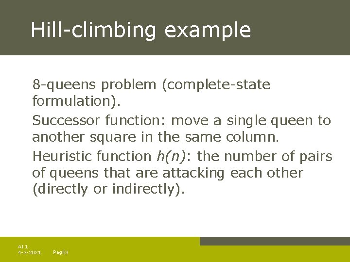
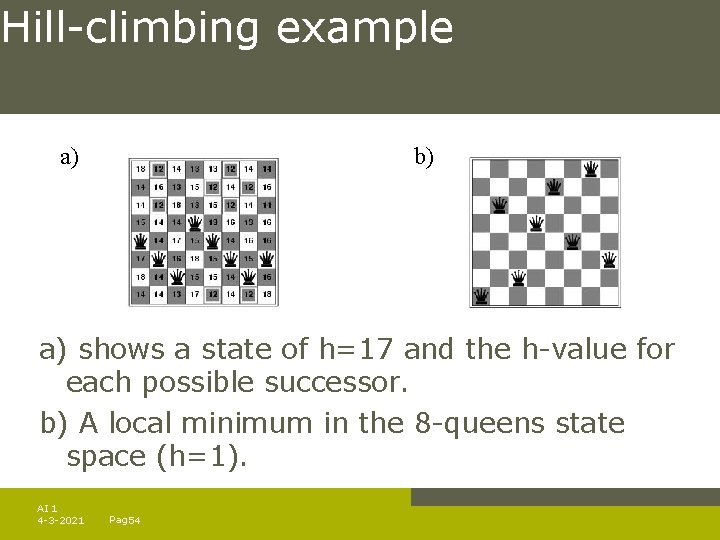
Hill-climbing example 8 -queens problem (complete-state formulation). Successor function: move a single queen to another square in the same column. Heuristic function h(n): the number of pairs of queens that are attacking each other (directly or indirectly). AI 1 4 -3 -2021 Pag. 53

Hill-climbing example a) b) a) shows a state of h=17 and the h-value for each possible successor. b) A local minimum in the 8 -queens state space (h=1). AI 1 4 -3 -2021 Pag. 54

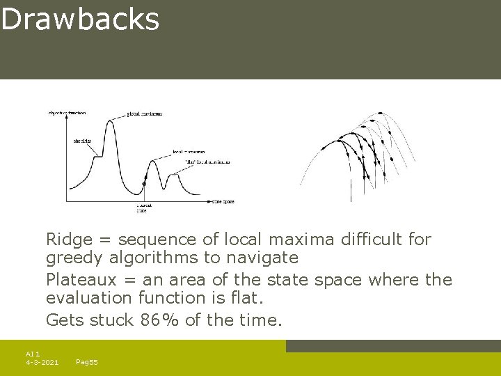
Drawbacks Ridge = sequence of local maxima difficult for greedy algorithms to navigate Plateaux = an area of the state space where the evaluation function is flat. Gets stuck 86% of the time. AI 1 4 -3 -2021 Pag. 55

Hill-climbing variations Stochastic hill-climbing – Random selection among the uphill moves. – The selection probability can vary with the steepness of the uphill move. First-choice hill-climbing – cfr. stochastic hill climbing by generating successors randomly until a better one is found. Random-restart hill-climbing – Tries to avoid getting stuck in local maxima. AI 1 4 -3 -2021 Pag. 56

Simulated annealing Escape local maxima by allowing “bad” moves. – Idea: but gradually decrease their size and frequency. Origin; metallurgical annealing Bouncing ball analogy: – Shaking hard (= high temperature). – Shaking less (= lower the temperature). If T decreases slowly enough, best state is reached. Applied for VLSI layout, airline scheduling, etc. AI 1 4 -3 -2021 Pag. 57

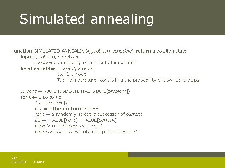
Simulated annealing function SIMULATED-ANNEALING( problem, schedule) return a solution state input: problem, a problem schedule, a mapping from time to temperature local variables: current, a node. next, a node. T, a “temperature” controlling the probability of downward steps current MAKE-NODE(INITIAL-STATE[problem]) for t 1 to ∞ do T schedule[t] if T = 0 then return current next a randomly selected successor of current ∆E VALUE[next] - VALUE[current] if ∆E > 0 then current next else current next only with probability e∆E /T AI 1 4 -3 -2021 Pag. 58

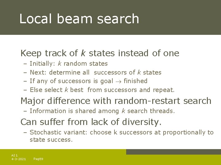
Local beam search Keep track of k states instead of one – – Initially: k random states Next: determine all successors of k states If any of successors is goal finished Else select k best from successors and repeat. Major difference with random-restart search – Information is shared among k search threads. Can suffer from lack of diversity. – Stochastic variant: choose k successors at proportionally to state success. AI 1 4 -3 -2021 Pag. 59

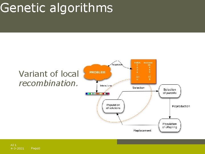
Genetic algorithms Variant of local beam search with sexual recombination. AI 1 4 -3 -2021 Pag. 60

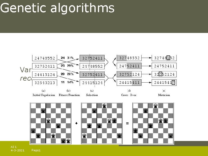
Genetic algorithms Variant of local beam search with sexual recombination. AI 1 4 -3 -2021 Pag. 61

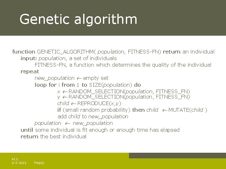
Genetic algorithm function GENETIC_ALGORITHM( population, FITNESS-FN) return an individual input: population, a set of individuals FITNESS-FN, a function which determines the quality of the individual repeat new_population empty set loop for i from 1 to SIZE(population) do x RANDOM_SELECTION(population, FITNESS_FN) y RANDOM_SELECTION(population, FITNESS_FN) child REPRODUCE(x, y) if (small random probability) then child MUTATE(child ) add child to new_population until some individual is fit enough or enough time has elapsed return the best individual AI 1 4 -3 -2021 Pag. 62

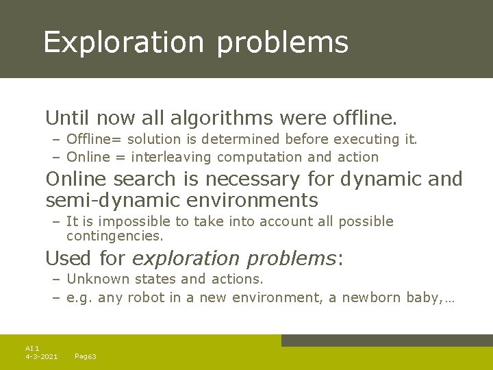
Exploration problems Until now all algorithms were offline. – Offline= solution is determined before executing it. – Online = interleaving computation and action Online search is necessary for dynamic and semi-dynamic environments – It is impossible to take into account all possible contingencies. Used for exploration problems: – Unknown states and actions. – e. g. any robot in a new environment, a newborn baby, … AI 1 4 -3 -2021 Pag. 63

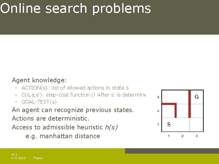
Online search problems Agent knowledge: – ACTION(s): list of allowed actions in state s – C(s, a, s’): step-cost function (! After s’ is determined) – GOAL-TEST(s) An agent can recognize previous states. Actions are deterministic. Access to admissible heuristic h(s) e. g. manhattan distance AI 1 4 -3 -2021 Pag. 64

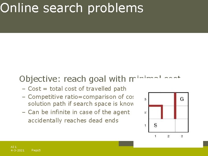
Online search problems Objective: reach goal with minimal cost – Cost = total cost of travelled path – Competitive ratio=comparison of cost with cost of the solution path if search space is known. – Can be infinite in case of the agent accidentally reaches dead ends AI 1 4 -3 -2021 Pag. 65

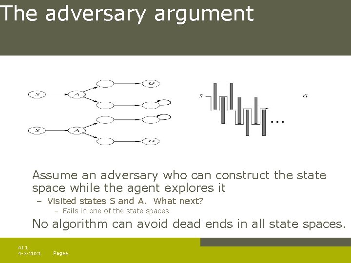
The adversary argument Assume an adversary who can construct the state space while the agent explores it – Visited states S and A. What next? – Fails in one of the state spaces No algorithm can avoid dead ends in all state spaces. AI 1 4 -3 -2021 Pag. 66

Online search agents The agent maintains a map of the environment. – Updated based on percept input. – This map is used to decide next action. Note difference with e. g. A* An online version can only expand the node it is physically in (local order) AI 1 4 -3 -2021 Pag. 67

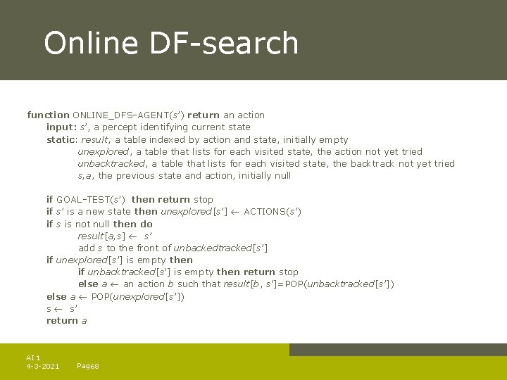
Online DF-search function ONLINE_DFS-AGENT(s’) return an action input: s’, a percept identifying current state static: result, a table indexed by action and state, initially empty unexplored, a table that lists for each visited state, the action not yet tried unbacktracked, a table that lists for each visited state, the backtrack not yet tried s, a, the previous state and action, initially null if GOAL-TEST(s’) then return stop if s’ is a new state then unexplored[s’] ACTIONS(s’) if s is not null then do result[a, s] s’ add s to the front of unbackedtracked[s’] if unexplored[s’] is empty then if unbacktracked[s’] is empty then return stop else a an action b such that result[b, s’]=POP(unbacktracked[s’]) else a POP(unexplored[s’]) s s’ return a AI 1 4 -3 -2021 Pag. 68

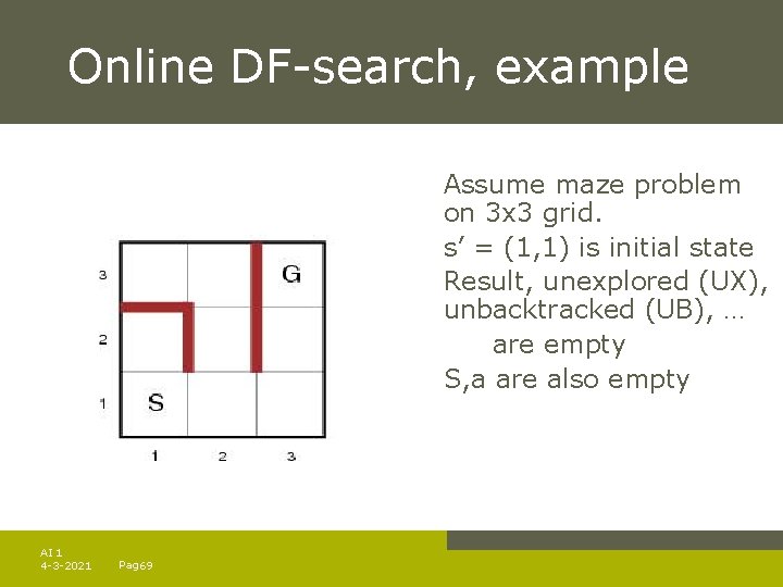
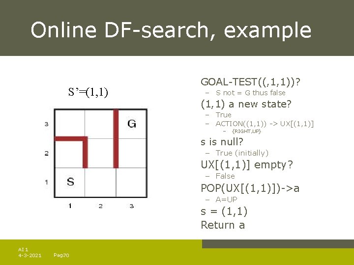
Online DF-search, example Assume maze problem on 3 x 3 grid. s’ = (1, 1) is initial state Result, unexplored (UX), unbacktracked (UB), … are empty S, a are also empty AI 1 4 -3 -2021 Pag. 69

Online DF-search, example S’=(1, 1) GOAL-TEST((, 1, 1))? – S not = G thus false (1, 1) a new state? – True – ACTION((1, 1)) -> UX[(1, 1)] – {RIGHT, UP} s is null? – True (initially) UX[(1, 1)] empty? – False POP(UX[(1, 1)])->a – A=UP s = (1, 1) Return a AI 1 4 -3 -2021 Pag. 70

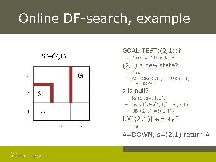
Online DF-search, example S’=(2, 1) GOAL-TEST((2, 1))? – S not = G thus false (2, 1) a new state? – True – ACTION((2, 1)) -> UX[(2, 1)] – S {DOWN} s is null? – false (s=(1, 1)) – result[UP, (1, 1)] <- (2, 1) – UB[(2, 1)]={(1, 1)} UX[(2, 1)] empty? – False A=DOWN, s=(2, 1) return A AI 1 4 -3 -2021 Pag. 71

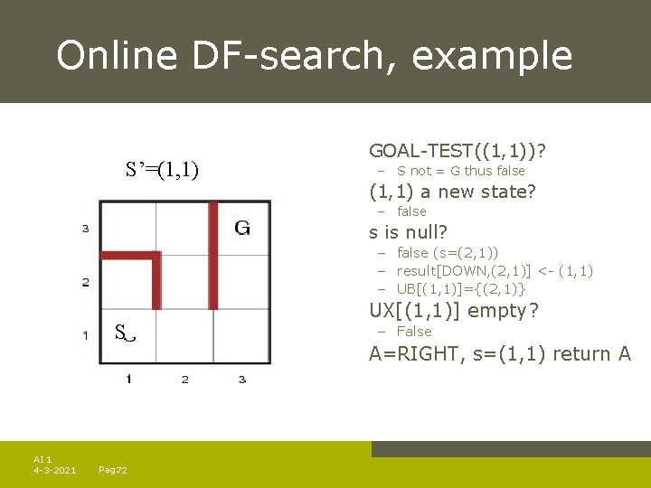
Online DF-search, example S’=(1, 1) GOAL-TEST((1, 1))? – S not = G thus false (1, 1) a new state? – false s is null? – false (s=(2, 1)) – result[DOWN, (2, 1)] <- (1, 1) – UB[(1, 1)]={(2, 1)} S AI 1 4 -3 -2021 Pag. 72 UX[(1, 1)] empty? – False A=RIGHT, s=(1, 1) return A

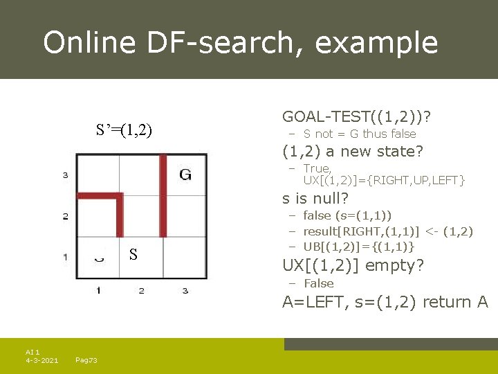
Online DF-search, example S’=(1, 2) GOAL-TEST((1, 2))? – S not = G thus false (1, 2) a new state? – True, UX[(1, 2)]={RIGHT, UP, LEFT} s is null? S – false (s=(1, 1)) – result[RIGHT, (1, 1)] <- (1, 2) – UB[(1, 2)]={(1, 1)} UX[(1, 2)] empty? – False A=LEFT, s=(1, 2) return A AI 1 4 -3 -2021 Pag. 73

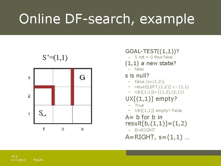
Online DF-search, example S’=(1, 1) GOAL-TEST((1, 1))? – (1, 1) a new state? – S false (s=(1, 2)) result[LEFT, (1, 2)] <- (1, 1) UB[(1, 1)]={(1, 2), (2, 1)} UX[(1, 1)] empty? – – false s is null? – – – S not = G thus false True UB[(1, 1)] empty? False A= b for b in result[b, (1, 1)]=(1, 2) – B=RIGHT A=RIGHT, s=(1, 1) … AI 1 4 -3 -2021 Pag. 74

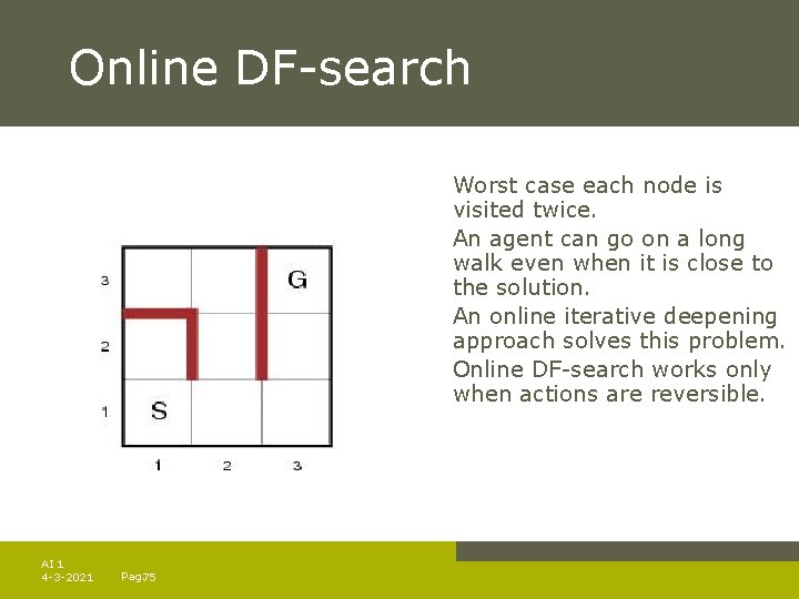
Online DF-search Worst case each node is visited twice. An agent can go on a long walk even when it is close to the solution. An online iterative deepening approach solves this problem. Online DF-search works only when actions are reversible. AI 1 4 -3 -2021 Pag. 75

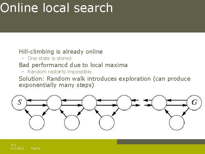
Online local search Hill-climbing is already online – One state is stored. Bad performancd due to local maxima – Random restarts impossible. Solution: Random walk introduces exploration (can produce exponentially many steps) AI 1 4 -3 -2021 Pag. 76

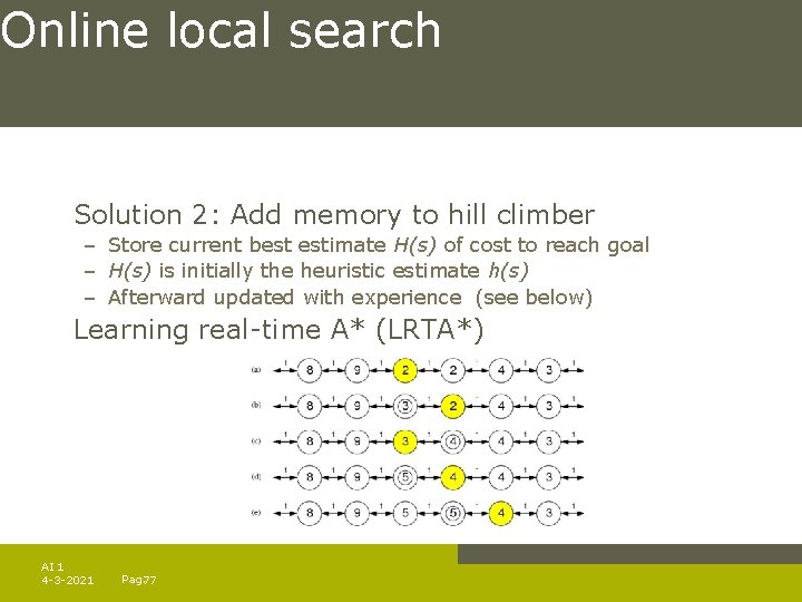
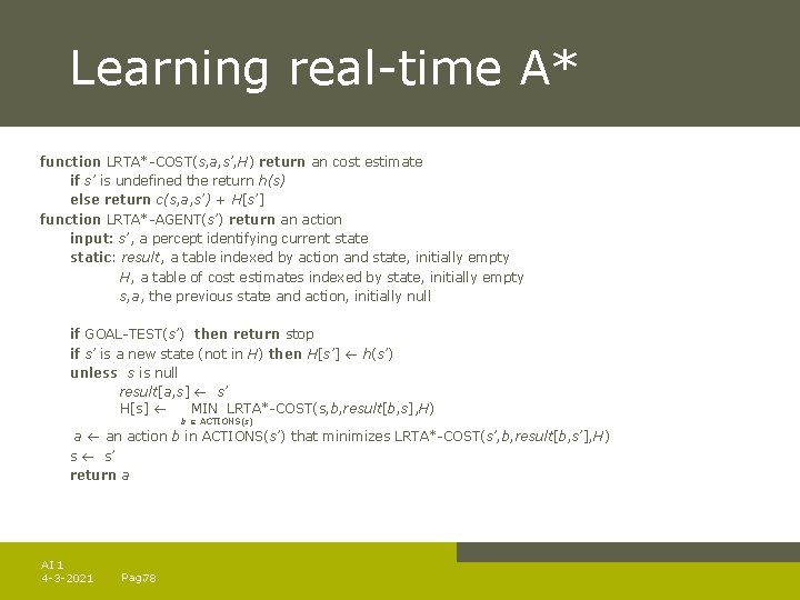
Online local search Solution 2: Add memory to hill climber – Store current best estimate H(s) of cost to reach goal – H(s) is initially the heuristic estimate h(s) – Afterward updated with experience (see below) Learning real-time A* (LRTA*) AI 1 4 -3 -2021 Pag. 77

Learning real-time A* function LRTA*-COST(s, a, s’, H) return an cost estimate if s’ is undefined the return h(s) else return c(s, a, s’) + H[s’] function LRTA*-AGENT(s’) return an action input: s’, a percept identifying current state static: result, a table indexed by action and state, initially empty H, a table of cost estimates indexed by state, initially empty s, a, the previous state and action, initially null if GOAL-TEST(s’) then return stop if s’ is a new state (not in H) then H[s’] h(s’) unless s is null result[a, s] s’ H[s] MIN LRTA*-COST(s, b, result[b, s], H) b ACTIONS(s) a an action b in ACTIONS(s’) that minimizes LRTA*-COST(s’, b, result[b, s’], H) s s’ return a AI 1 4 -3 -2021 Pag. 78