Informed search algorithms Chapter 4 Outline Bestfirst search

Informed search algorithms Chapter 4

Outline • • Best-first search Greedy best-first search A* search Heuristics Local search algorithms Hill-climbing search Simulated annealing search Genetic algorithms
 for each node – estimate")
Best-first search • Idea: use an evaluation function f(n) for each node – estimate of "desirability" Expand most desirable unexpanded node • Implementation: Order the nodes in fringe in decreasing order of desirability • Special cases: – greedy best-first search

Romania with step costs in km
 = h(n) (heuristic) = estimate of cost")
Greedy best-first search • Evaluation function f(n) = h(n) (heuristic) = estimate of cost from n to goal • e. g. , h. SLD(n) = straight-line distance from n to Bucharest • Greedy best-first search expands the node that appears to be closest to goal

Greedy best-first search example

Greedy best-first search example

Greedy best-first search example

Greedy best-first search example
 for some problems • 8 -puzzle – W(n): number of misplaced tiles –")
H(n) for some problems • 8 -puzzle – W(n): number of misplaced tiles – Manhatten distance – Gaschnig’s heuristic • 8 -queen – Number of future feasible slots – Min number of feasible slots in a row • Travelling salesperson – Minimum spanning tree
 search h(n) = number of misplaced tiles")
Best first (Greedy) search h(n) = number of misplaced tiles

Properties of greedy best-first search • Complete? No – can get stuck in loops, e. g. , Iasi Neamt • Time? O(bm), but a good heuristic can give dramatic improvement • Space? O(bm) -- keeps all nodes in memory

Problems with Greedy Search • Not complete • • Get stuck on local minimas and plateaus Irrevocable Infinite loops Can we incorporate heuristics in systematic search?

Modified heuristic for 8 -puzzle

Traveling salesman problem Given a weighted directed graph G = <V, E, w>, find a sequence of nodes that starts and ends in the same node and visits all the nodes at least once. The total cost of the path should be minimized. A near-optimal solution to the geometric TSP problem

Subset selection problem Given a list of numbers S = {x 1, …, xn}, and a target t, find a subset I of S whose sum is as large as possible, but not exceed t. Questions: 1) How do we model these problems as search problems? 2) What heuristic h(. ) can you suggest for the problems?

State space for TSP and subset sum problem TSP: State-space representation: Each node represents a partial tour. Children of a node extend the path of length k into a path of length k + 1 Subset sum: at each level one element is considered (left child corresponds to excluding the element; right child corresponds to including it. )

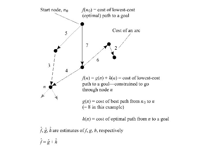
A* search • Idea: avoid expanding paths that are already expensive – Evaluation function f(n) = g(n) + h(n) • g(n) = cost so far to reach n • h(n) = estimated cost from n to goal • f(n) = estimated total cost of path through n to goal

A* search example

A* search example

A* search example

A* search example

A* search example

A* search example

Algorithm A* Input: a search graph with cost on the arcs Output: the minimal cost path from start node to a goal node. 1. Put the start node s on OPEN. 2. If OPEN is empty, exit with failure 3. Remove from OPEN and place on CLOSED a node n having minimum f. 4. If n is a goal node exit successfully with a solution path obtained by tracing back the pointers from n to s. 5. Otherwise, expand n generating its children and directing pointers from each child node to n. • For every child node n’ do – evaluate h(n’) and compute f(n’) = g(n’) +h(n’)= g(n)+c(n, n’)+h(n) – If n’ is already on OPEN or CLOSED compare its new f with the old f and attach the lowest f to n’. – put n’ with its f value in the right order in OPEN 6. Go to step 2.
 is admissible if for every node n, h(n)")
Admissible heuristics • A heuristic h(n) is admissible if for every node n, h(n) ≤ h*(n), where h*(n) is the true cost to reach the goal state from n. • An admissible heuristic never overestimates the cost to reach the goal, i. e. , it is optimistic Example: h. SLD(n) (never overestimates the actual road distance)
 • Suppose some suboptimal goal G 2 has been generated")
Optimality of A* (proof) • Suppose some suboptimal goal G 2 has been generated and is in the fringe. Let n be an unexpanded node in the fringe such that n is on a shortest path to an optimal goal G. f(G 2) = g(G 2) > g(G) f(G) = g(G) f(G 2) > f(G) since h(G 2) = 0 since G 2 is suboptimal since h(G) = 0 from above
 • Suppose some suboptimal goal G 2 has been generated")
Optimality of A* (proof) • Suppose some suboptimal goal G 2 has been generated and is in the fringe. Let n be an unexpanded node in the fringe such that n is on a shortest path to an optimal goal G. • • f(G 2) > f(G) from above h(n) ≤ h*(n) since h is admissible g(n) + h(n) ≤ g(n) + h*(n) f(n) ≤ f(G) Hence f(G ) > f(n), and A* will never select G for expansion
 (Hart, Nillson and Raphael, 1968) A* always terminates with")
A* termination • Theorem (completeness) (Hart, Nillson and Raphael, 1968) A* always terminates with a solution path if • costs on arcs are positive, above epsilon • branching degree is finite. • Proof: The evaluation function f of nodes expanded must increase eventually until all the nodes on an optimal path are expanded.

Consistent heuristics • A heuristic is consistent if for every node n, every successor n' of n generated by any action a, • h(n) ≤ c(n, a, n') + h(n') • If h is consistent, we have f(n') = g(n') + h(n') = g(n) + c(n, a, n') + h(n') ≥ g(n) + h(n) = f(n) • i. e. , f(n) is non-decreasing along any path.

Optimality of A* • A* expands nodes in order of increasing f value • Gradually adds "f-contours" of nodes • Contour i has all nodes with f=fi, where fi < fi+1

Properties of A* • Complete? Yes (unless there are infinitely many nodes with f ≤ f(G) ) • Time? Exponential • Space? Keeps all nodes in memory
 = number")
Admissible heuristics E. g. , for the 8 -puzzle: • h 1(n) = number of misplaced tiles • h 2(n) = total Manhattan distance (i. e. , no. of squares from desired location of each tile) • h 1(S) = ?
 = number")
Admissible heuristics E. g. , for the 8 -puzzle: • h 1(n) = number of misplaced tiles • h 2(n) = total Manhattan distance (i. e. , no. of squares from desired location of each tile) • h 1(S) = 8 • h (S) = 3+1+2+2+2+3+3+2 = 18
 ≥ h 1(n) for all n (both admissible) then")
Dominance • If h 2(n) ≥ h 1(n) for all n (both admissible) then h 2 dominates h 1 h 2 is better for search
")
Effectiveness of A* Search Algorithm Average number of nodes expanded d IDS A*(h 1) A*(h 2) 2 10 6 6 4 112 13 12 8 6384 39 25 12 364404 227 73 14 3473941 539 113 20 ------7276 676 Average over 100 randomly generated 8 -puzzle problems h 1 = number of tiles in the wrong position h 2 = sum of Manhattan distances

Relaxed problems • A problem with fewer restrictions on the actions is called a relaxed problem • The cost of an optimal solution to a relaxed problem is an admissible heuristic for the original problem • If the rules of the 8 -puzzle are relaxed so that a tile can move anywhere, then h 1(n) gives the shortest solution • If the rules are relaxed so that a tile can move to any adjacent square, then h 2(n) gives the shortest solution

Local search algorithms • In many optimization problems, the path to the goal is irrelevant; the goal state itself is the solution • State space = set of complete configurations • Find configuration satisfying constraints, e. g. , nqueens • In such cases, we can use local search algorithms • keep a single "current" state, try to improve it

Example: subset sum problem

Hill-climbing search • "Like climbing Everest in thick fog with amnesia"

Hill-climbing search • Problem: depending on initial state, can get stuck in local maxima

Hill-climbing search: 8 -queens problem • h = number of pairs of queens that are attacking each other, either directly or indirectly • h = 17 for the above state

Hill-climbing search: 8 -queens problem • A local minimum with h = 1

Simulated annealing search • Idea: escape local maxima by allowing some "bad" moves but gradually decrease their frequency

Properties of simulated annealing search • It can be proved: “If T decreases slowly enough, then simulated annealing search will find a global optimum with probability approaching 1. ” • Widely used in VLSI layout, airline scheduling, etc.

Relationships among search algorithms

Inventing Heuristics automatically • Examples of Heuristic Functions for A* How can we invent admissible heuristics in general? – look at “relaxed” problem where constraints are removed • e. g. . , we can move in straight lines between cities • e. g. . , we can move tiles independently of each other
 • How did we – find h 1 and h")
Inventing Heuristics Automatically (continued) • How did we – find h 1 and h 2 for the 8 -puzzle? – verify admissibility? – prove that air-distance is admissible? MST admissible? • Hypothetical answer: – Heuristic are generated from relaxed problems – Hypothesis: relaxed problems are easier to solve • In relaxed models the search space has more operators, or more directed arcs • Example: 8 puzzle: – A tile can be moved from A to B if A is adjacent to B and B is clear – We can generate relaxed problems by removing one or more of the conditions • A tile can be moved from A to B if A is adjacent to B • . . . if B is blank • A tile can be moved from A to B.
 • Example: TSP • Find a tour. A tour is: –")
Generating heuristics (continued) • Example: TSP • Find a tour. A tour is: – 1. A graph – 2. Connected – 3. Each node has degree 2. • Eliminating 2 yields MST.

Automating Heuristic generation Operators: – Pre-conditions, add-list, delete list 8 -puzzle example: – On(x, y), clear(y), adj(y, z) , tiles x 1, …, x 8 • States: conjunction of predicates: – On(x 1, c 1), on(x 2, c 2)…. on(x 8, c 8), clear(c 9) • Move(x, c 1, c 2) (move tile x from location c 1 to location c 2) – Pre-cond: on(x 1. c 1), clear(c 2), adj(c 1, c 2) – Add-list: on(x 1, c 2), clear(c 1) – Delete-list: on(x 1, c 1), clear(c 2) Relaxation: 1. Remove from pre-cond: clear(c 2), adj(c 2, c 3) #misplaced tiles 2. Remove clear(c 2) manhatten distance 3. Remove adj(c 2, c 3) h 3, a new procedure that transfer to the empty location a tile appearing there in the goal

Pattern Databases • For sliding tiles and Rubic’s cube • For a subset of the tiles compute shortest path to the goal using breadth-first search • For 15 puzzles, if we have 7 fringe tiles and one blank, the number of patterns to store are 16!/(16 -8)! = 518, 918, 400. • For each table entry we store the shortest number of moves to the goal from the current location.

Problem-reduction representations AND/OR search spaces • Symbolic integration

AND/OR Graphs • Nodes represent subproblems – – And links represent subproblem decompositions OR links represent alternative solutions Start node is initial problem Terminal nodes are solved subproblems • Solution graph – It is an AND/OR subgraph such that: – 1. It contains the start node – 2. All it terminal nodes (nodes with no successors) are solved primitive problems – 3. If it contains an AND node L, it must contain the entire group of AND links that leads to children of L.

Algorithms searching AND/OR graphs • All algorithms generalize using hyper-arc suscessors rather than simple arcs. • AO*: is A* that searches AND/OR graphs for a solution subgraph. • The cost of a solution graph is the sum cost of it arcs. It can be defined recursively as: k(n, N) = c_n+k(n 1, N)+…k(n_k, N) • h*(n) is the cost of an optimal solution graph from n to a set of goal nodes • h(n) is an admissible heuristic for h*(n) • Monotonicity: • h(n)<= c+h(n 1)+…h(nk) where n 1, …nk are successors of n • AO* is guaranteed to find an optimal solution when it terminates if the heuristic function is admissible

Summary • In practice we often want the goal with the minimum cost path • Exhaustive search is impractical except on small problems • Heuristic estimates of the path cost from a node to the goal can be efficient in reducing the search space. • The A* algorithm combines all of these ideas with admissible heuristics (which underestimate) , guaranteeing optimality. • Properties of heuristics: – admissibility, monotonicity, dominance, accuracy • Simulated annealing, local search – are heuristics that usually produce sub-optimal solutions since they may terminate at local optimal solution.
- Slides: 56