Implementation of 2 D FFT on the Cell

Implementation of 2 -D FFT on the Cell Broadband Engine Architecture William Lundgren (wlundgren@gedae. com, Gedae), Kerry Barnes (Gedae), James Steed (Gedae) HPEC 2009

Introduction Processing is either limited by memory or CPU bandwidth – Challenge is to achieve the practical limit of processing – Large 2 -D FFTs are limited by memory bandwidth Automating details of implementation provides developer with more opportunity to optimize structure of algorithm Cell Broadband Engine is a good platform for studying efficient use of memory bandwidth – Data movements are exposed and can be controlled – Cache managers hide the data movement Intel X 86 & IBM Power processor clusters, Larrabee, Tilera, etc. have similar challenges 2

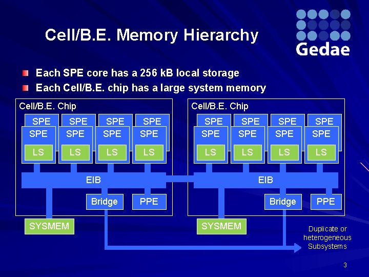
Cell/B. E. Memory Hierarchy Each SPE core has a 256 k. B local storage Each Cell/B. E. chip has a large system memory Cell/B. E. Chip SPE SPE LS LS SPE SPE LS LS EIB Bridge SYSMEM SPE SPE LS LS Bridge PPE EIB PPE SYSMEM Duplicate or heterogeneous Subsystems 3

Effect of Tile Size on Throughput # Procs (Times are measured within Gedae)

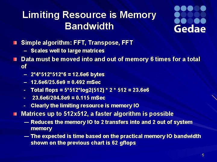
Limiting Resource is Memory Bandwidth Simple algorithm: FFT, Transpose, FFT – Scales well to large matrices Data must be moved into and out of memory 6 times for a total of – – - 2*4*512*6 = 12. 6 e 6 bytes 12. 6 e 6/25. 6 e 9 = 0. 492 m. Sec Total flops = 5*512*log 2(512) * 2 * 512 = 23. 6 e 6/204. 8 e 9 = 0. 115 m. Sec Clearly the limiting resource is memory IO Matrices up to 512 x 512, a faster algorithm is possible ― Reduces the memory IO to 2 transfers into and 2 out of system memory ― The expected is time based on the practical memory IO bandwidth shown on the previous chart is 62 gflops 5

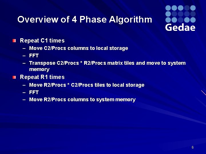
Overview of 4 Phase Algorithm Repeat C 1 times – – – Move C 2/Procs columns to local storage FFT Transpose C 2/Procs * R 2/Procs matrix tiles and move to system memory Repeat R 1 times – – – Move R 2/Procs * C 2/Procs tiles to local storage FFT Move R 2/Procs columns to system memory 6

Optimization of Data Movement We know that to achieve optimal performance we must use buffers with row length >= 2048 bytes Complexity beyond the reach of many programmers Approach: Use Idea Language (Copyright Gedae, Inc. ) to design the data organization and movement among memories Implement on Cell processor using Gedae DF Future implementation will be fully automated from Idea design The following charts show the algorithm design using the Idea Language and implementation and diagrams Multicores require the introduction of fundamentally new automation. 7

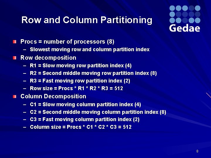
Row and Column Partitioning Procs = number of processors (8) – Slowest moving row and column partition index Row decomposition – – R 1 = Slow moving row partition index (4) R 2 = Second middle moving row partition index (8) R 3 = Fast moving row partition index (2) Row size = Procs * R 1 * R 2 * R 3 = 512 Column Decomposition – – C 1 = Slow moving column partition index (4) C 2 = Second middle moving column partition index (8) C 3 = Fast moving column partition index (2) Column size = Procs * C 1 * C 2 * C 3 = 512 8

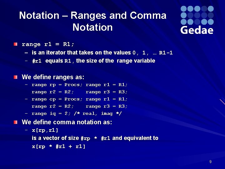
Notation – Ranges and Comma Notation range r 1 = R 1; – is an iterator that takes on the values 0, 1, … R 1 -1 – #r 1 equals R 1, the size of the range variable We define ranges as: – range – range rp r 2 cp r 2 iq = = = Procs; range r 1 = R 1; R 2; range r 3 = R 3; 2; /* real, imag */ We define comma notation as: – x[rp, r 1] is a vector of size #rp * #r 1 and equivalent to x[rp * #r 1 + r 1] 9

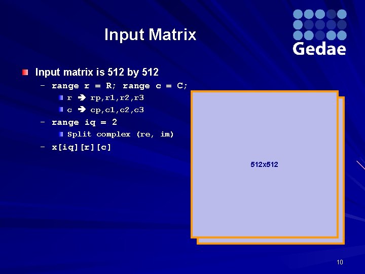
Input Matrix Input matrix is 512 by 512 – range r = R; range c = C; r rp, r 1, r 2, r 3 c cp, c 1, c 2, c 3 – range iq = 2 Split complex (re, im) – x[iq][r][c] 512 x 512 10

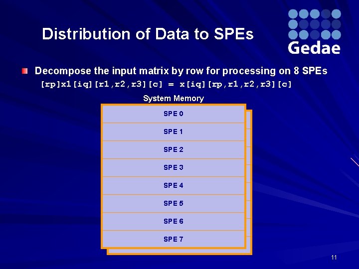
Distribution of Data to SPEs Decompose the input matrix by row for processing on 8 SPEs [rp]x 1[iq][r 1, r 2, r 3][c] = x[iq][rp, r 1, r 2, r 3][c] System Memory SPE 0 SPE 1 SPE 2 SPE 3 SPE 4 SPE 5 SPE 6 SPE 7 11

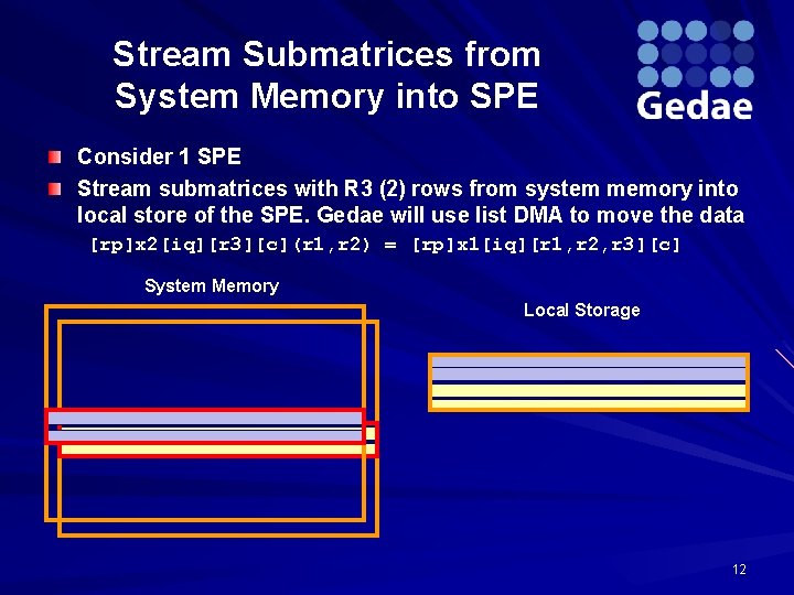
Stream Submatrices from System Memory into SPE Consider 1 SPE Stream submatrices with R 3 (2) rows from system memory into local store of the SPE. Gedae will use list DMA to move the data [rp]x 2[iq][r 3][c](r 1, r 2) = [rp]x 1[iq][r 1, r 2, r 3][c] System Memory Local Storage 12

FFT Processing Process Submatrices by Computing FFT on Each Row – [rp]x 3[r 3][iq][c]= fft([rp]x 2[iq][r 3]) – Since the [c] dimension is dropped from the argument to the fft function it is being passed a complete row (vector). – Stream indices are dropped. The stream processing is automatically implemented by Gedae. Each sub matrix contains 2 rows of real and 2 rows of imaginary data. FFT Processing Notice that the real and imaginary data has been interleaved to keep each submatrix in contiguous memory. 13

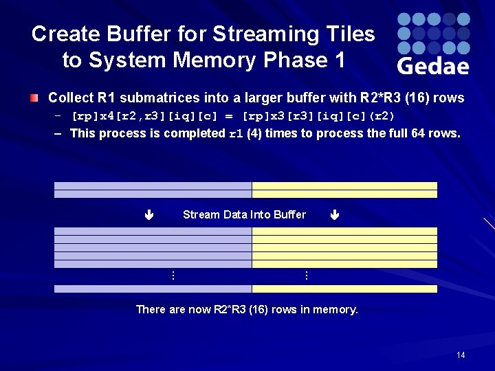
Create Buffer for Streaming Tiles to System Memory Phase 1 Collect R 1 submatrices into a larger buffer with R 2*R 3 (16) rows – [rp]x 4[r 2, r 3][iq][c] = [rp]x 3[r 3][iq][c](r 2) – This process is completed r 1 (4) times to process the full 64 rows. Stream Data Into Buffer … … There are now R 2*R 3 (16) rows in memory. 14

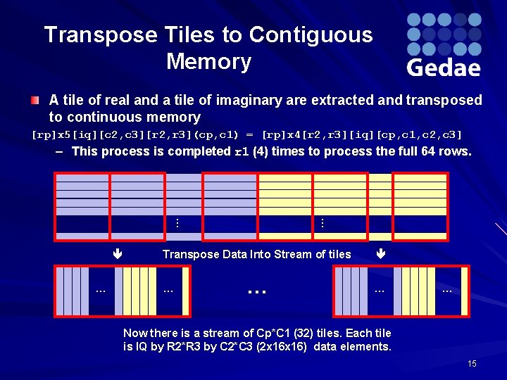
Transpose Tiles to Contiguous Memory A tile of real and a tile of imaginary are extracted and transposed to continuous memory [rp]x 5[iq][c 2, c 3][r 2, r 3](cp, c 1) = [rp]x 4[r 2, r 3][iq][cp, c 1, c 2, c 3] – This process is completed r 1 (4) times to process the full 64 rows. … … … Transpose Data Into Stream of tiles … … Now there is a stream of Cp*C 1 (32) tiles. Each tile is IQ by R 2*R 3 by C 2*C 3 (2 x 16) data elements. 15

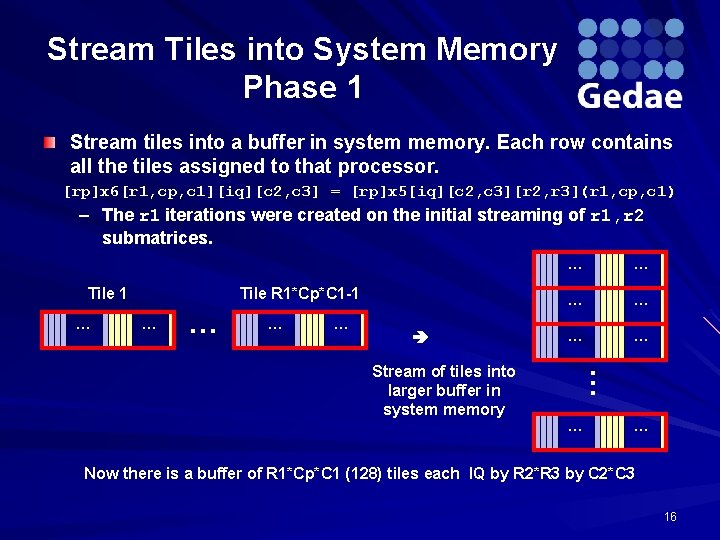
Stream Tiles into System Memory Phase 1 Stream tiles into a buffer in system memory. Each row contains all the tiles assigned to that processor. [rp]x 6[r 1, cp, c 1][iq][c 2, c 3] = [rp]x 5[iq][c 2, c 3][r 2, r 3](r 1, cp, c 1) – The r 1 iterations were created on the initial streaming of r 1, r 2 submatrices. Tile 1 … Tile R 1*Cp*C 1 -1 … … … … … Stream of tiles into larger buffer in system memory … … … Now there is a buffer of R 1*Cp*C 1 (128) tiles each IQ by R 2*R 3 by C 2*C 3 16

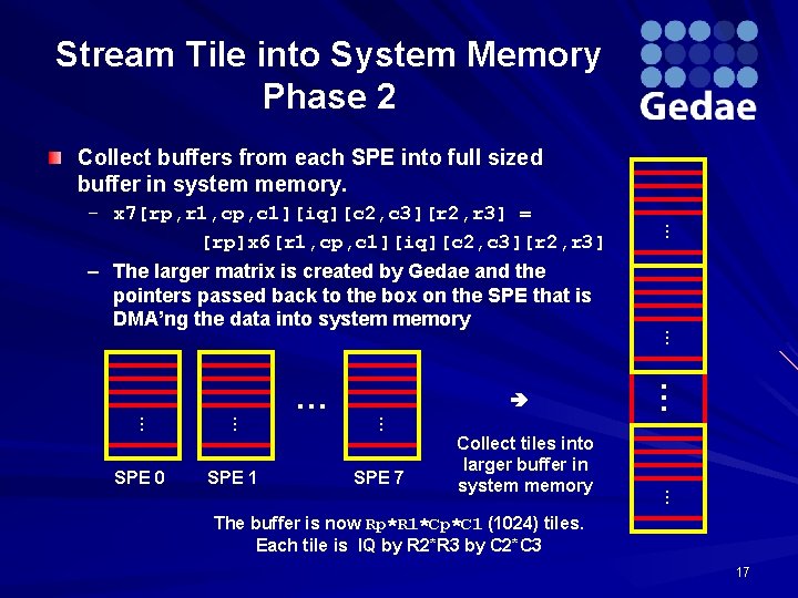
Stream Tile into System Memory Phase 2 Collect buffers from each SPE into full sized buffer in system memory. SPE 7 … Collect tiles into larger buffer in system memory … SPE 1 … … … SPE 0 … … … – x 7[rp, r 1, cp, c 1][iq][c 2, c 3][r 2, r 3] = [rp]x 6[r 1, cp, c 1][iq][c 2, c 3][r 2, r 3] – The larger matrix is created by Gedae and the pointers passed back to the box on the SPE that is DMA’ng the data into system memory The buffer is now Rp*R 1*Cp*C 1 (1024) tiles. Each tile is IQ by R 2*R 3 by C 2*C 3 17

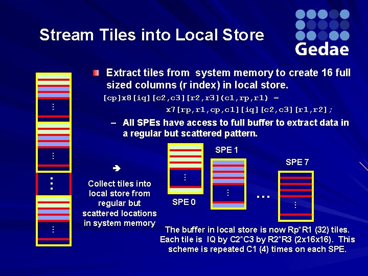
Stream Tiles into Local Store Extract tiles from system memory to create 16 full sized columns (r index) in local store. … [cp]x 8[iq][c 2, c 3][r 2, r 3](c 1, rp, r 1) = x 7[rp, r 1, cp, c 1][iq][c 2, c 3][r 1, r 2]; – All SPEs have access to full buffer to extract data in a regular but scattered pattern. … SPE 1 SPE 7 … … … SPE 0 … … … Collect tiles into local store from regular but scattered locations in system memory The buffer in local store is now Rp*R 1 (32) tiles. Each tile is IQ by C 2*C 3 by R 2*R 3 (2 x 16). This scheme is repeated C 1 (4) times on each SPE.

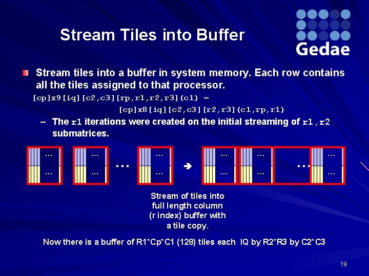
Stream Tiles into Buffer Stream tiles into a buffer in system memory. Each row contains all the tiles assigned to that processor. [cp]x 9[iq][c 2, c 3][rp, r 1, r 2, r 3](c 1) = [cp]x 8[iq][c 2, c 3][r 2, r 3](c 1, rp, r 1) – The r 1 iterations were created on the initial streaming of r 1, r 2 submatrices. … … … … Stream of tiles into full length column (r index) buffer with a tile copy. Now there is a buffer of R 1*Cp*C 1 (128) tiles each IQ by R 2*R 3 by C 2*C 3 19

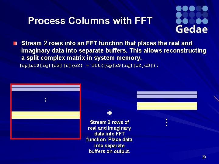
Process Columns with FFT Stream 2 rows into an FFT function that places the real and imaginary data into separate buffers. This allows reconstructing a split complex matrix in system memory. [cp]x 10[iq][c 3][r](c 2) = fft([cp]x 9[iq][c 2, c 3]); … Stream 2 rows of real and imaginary data into FFT function. Place data into separate buffers on output. … 20

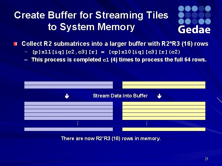
Create Buffer for Streaming Tiles to System Memory Collect R 2 submatrices into a larger buffer with R 2*R 3 (16) rows – [p]x 11[iq][c 2, c 3][r] = [cp]x 10[iq][c 3][r](c 2) – This process is completed c 1 (4) times to process the full 64 rows. Stream Data Into Buffer … … There are now R 2*R 3 (16) rows in memory. 21

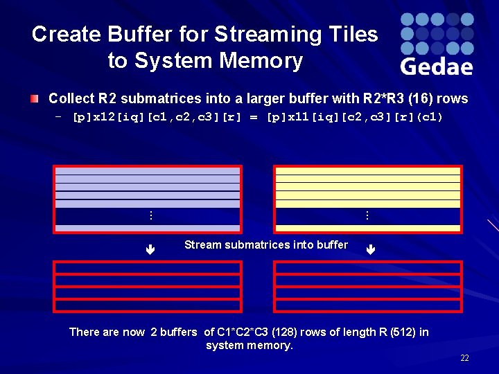
Create Buffer for Streaming Tiles to System Memory Collect R 2 submatrices into a larger buffer with R 2*R 3 (16) rows – [p]x 12[iq][c 1, c 2, c 3][r] = [p]x 11[iq][c 2, c 3][r](c 1) … … Stream submatrices into buffer There are now 2 buffers of C 1*C 2*C 3 (128) rows of length R (512) in system memory. 22

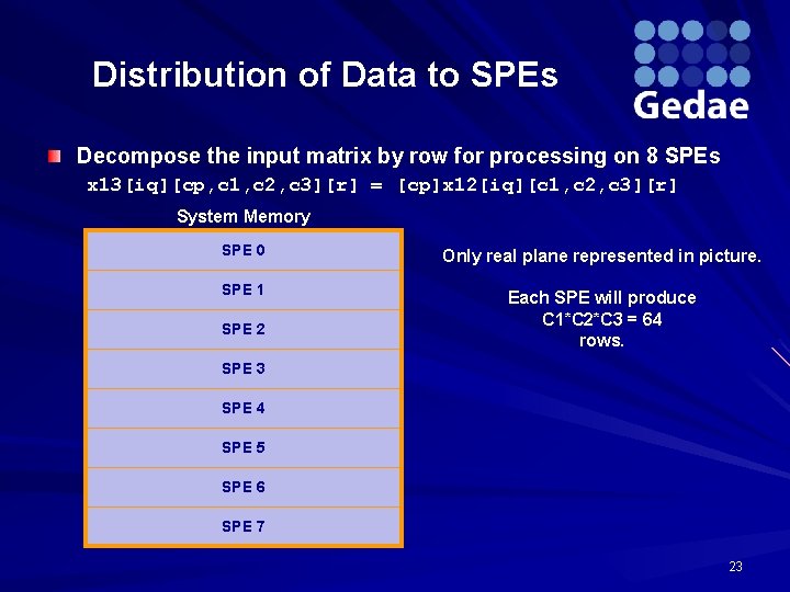
Distribution of Data to SPEs Decompose the input matrix by row for processing on 8 SPEs x 13[iq][cp, c 1, c 2, c 3][r] = [cp]x 12[iq][c 1, c 2, c 3][r] System Memory SPE 0 Only real plane represented in picture. SPE 1 Each SPE will produce C 1*C 2*C 3 = 64 rows. SPE 2 SPE 3 SPE 4 SPE 5 SPE 6 SPE 7 23

Output Matrix Output matrix is 512 by 512 – y[iq][c][r] 512 x 512 24

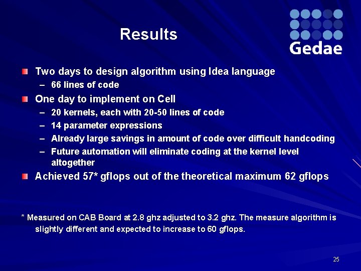
Results Two days to design algorithm using Idea language – 66 lines of code One day to implement on Cell – – 20 kernels, each with 20 -50 lines of code 14 parameter expressions Already large savings in amount of code over difficult handcoding Future automation will eliminate coding at the kernel level altogether Achieved 57* gflops out of theoretical maximum 62 gflops * Measured on CAB Board at 2. 8 ghz adjusted to 3. 2 ghz. The measure algorithm is slightly different and expected to increase to 60 gflops. 25

Gedae Status 12 months into an 18/20 month repackaging of Gedae – Introduced algebraic features of the Idea language used to design this algorithm – Completed support for hierarchical memory – Embarking now on code overlays and large scale heterogeneous systems – Will reduce memory footprint to enable 1024 x 1024 2 D FFT 26