Parallel FFT Sathish Vadhiyar Sequential FFT Quick Review

Parallel FFT Sathish Vadhiyar

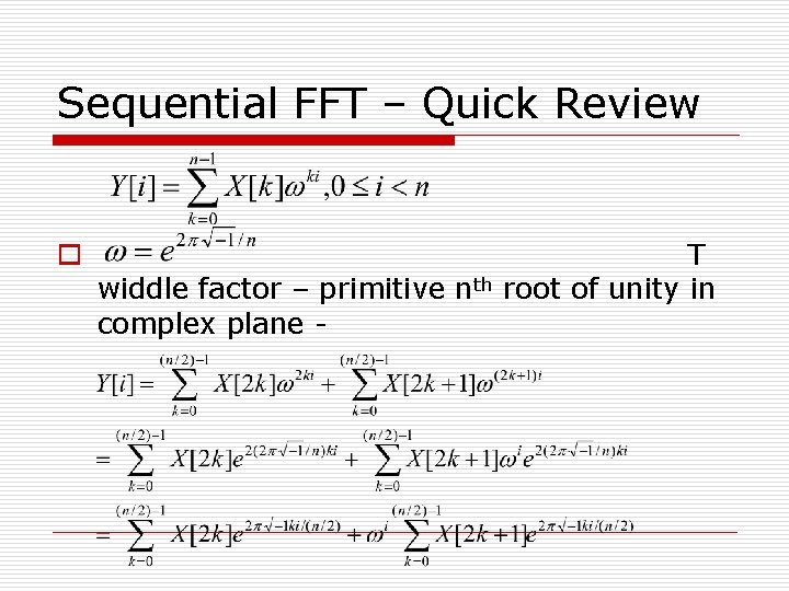
Sequential FFT – Quick Review o widdle factor – primitive nth complex plane - T root of unity in

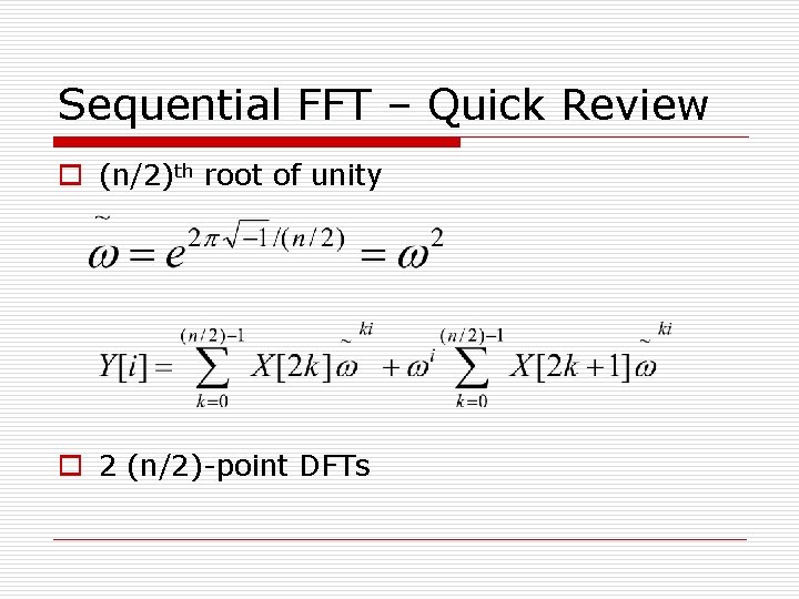
Sequential FFT – Quick Review o (n/2)th root of unity o 2 (n/2)-point DFTs

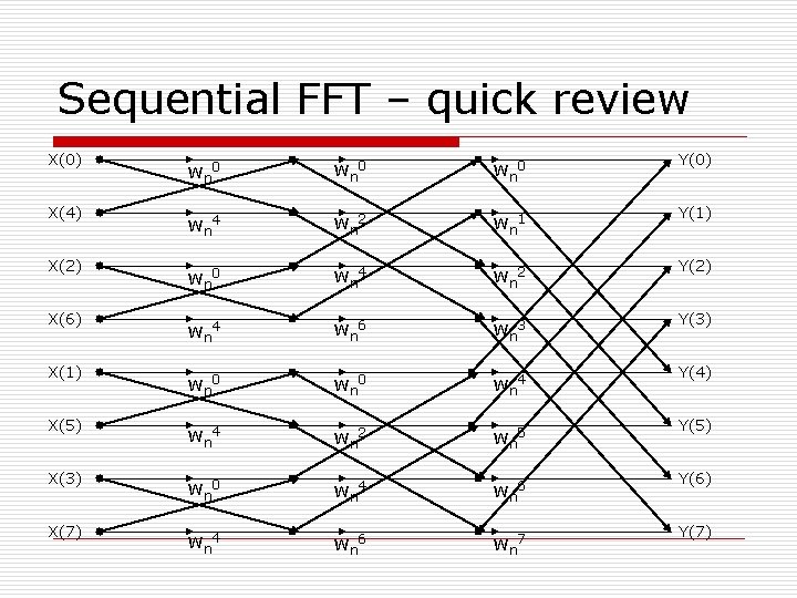
Sequential FFT – quick review X(0) wn 0 Y(0) wn 4 wn 2 wn 1 Y(1) wn 0 wn 4 wn 2 Y(2) wn 4 wn 6 wn 3 Y(3) wn 0 wn 4 X(5) wn 4 wn 2 wn 5 X(3) wn 0 wn 4 wn 6 X(7) wn 4 wn 6 wn 7 X(4) X(2) X(6) X(1) Y(4) Y(5) Y(6) Y(7)

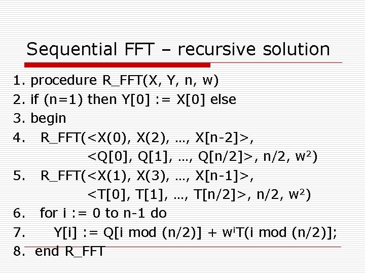
Sequential FFT – recursive solution 1. procedure R_FFT(X, Y, n, w) 2. if (n=1) then Y[0] : = X[0] else 3. begin 4. R_FFT(<X(0), X(2), …, X[n-2]>, <Q[0], Q[1], …, Q[n/2]>, n/2, w 2) 5. R_FFT(<X(1), X(3), …, X[n-1]>, <T[0], T[1], …, T[n/2]>, n/2, w 2) 6. for i : = 0 to n-1 do 7. Y[i] : = Q[i mod (n/2)] + wi. T(i mod (n/2)]; 8. end R_FFT

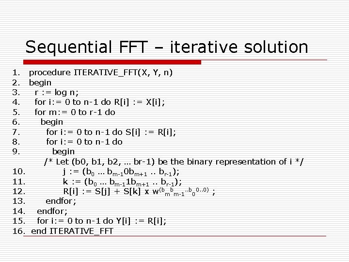
Sequential FFT – iterative solution 1. 2. 3. 4. 5. 6. 7. 8. 9. 10. 11. 12. 13. 14. 15. 16. procedure ITERATIVE_FFT(X, Y, n) begin r : = log n; for i: = 0 to n-1 do R[i] : = X[i]; for m: = 0 to r-1 do begin for i: = 0 to n-1 do S[i] : = R[i]; for i: = 0 to n-1 do begin /* Let (b 0, b 1, b 2, … br-1) be the binary representation of i */ j : = (b 0 … bm-10 bm+1. . br-1); k : = (b 0 … bm-11 bm+1. . br-1); R[i] : = S[j] + S[k] x w(bmbm-1. . b 00. . 0) ; endfor; for i: = 0 to n-1 do Y[i] : = R[i]; end ITERATIVE_FFT

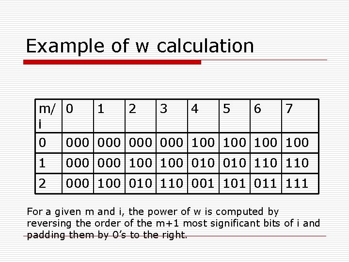
Example of w calculation m/ 0 1 2 3 4 5 6 7 i 0 000 000 100 100 1 000 100 010 110 2 000 100 010 110 001 101 011 111 For a given m and i, the power of w is computed by reversing the order of the m+1 most significant bits of i and padding them by 0’s to the right.

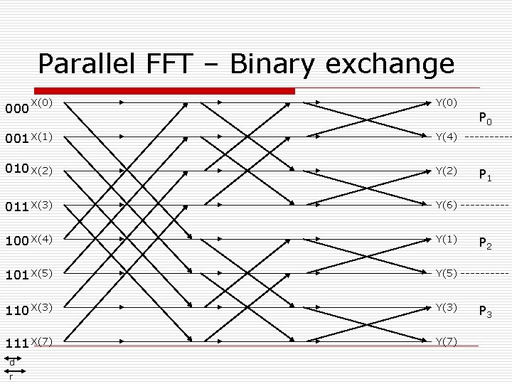
Parallel FFT – Binary exchange 000 X(0) Y(0) P 0 001 X(1) Y(4) 010 X(2) Y(2) 011 X(3) Y(6) 100 X(4) Y(1) 101 X(5) Y(5) 110 X(3) Y(3) 111 X(7) Y(7) d r P 1 P 2 P 3

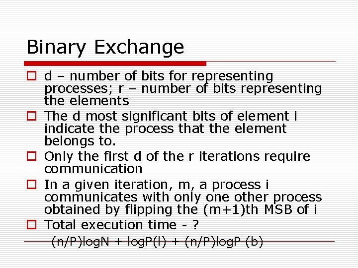
Binary Exchange o d – number of bits for representing processes; r – number of bits representing the elements o The d most significant bits of element i indicate the process that the element belongs to. o Only the first d of the r iterations require communication o In a given iteration, m, a process i communicates with only one other process obtained by flipping the (m+1)th MSB of i o Total execution time - ? (n/P)log. N + log. P(l) + (n/P)log. P (b)

Parallel FFT – 2 D Transpose P 0 P 1 P 2 P 3 0 1 2 3 4 5 6 7 8 9 10 11 12 13 14 15 m=0 m=1 Phase 1 – FFTs along columns

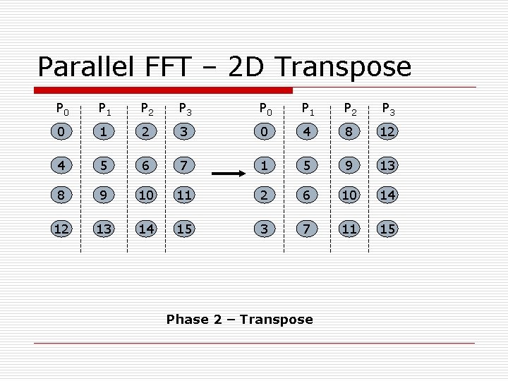
Parallel FFT – 2 D Transpose P 0 P 1 P 2 P 3 0 1 2 3 0 4 8 12 4 5 6 7 1 5 9 13 8 9 10 11 2 6 10 14 12 13 14 15 3 7 11 15 Phase 2 – Transpose

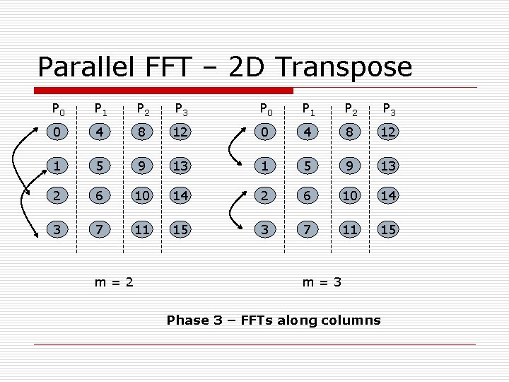
Parallel FFT – 2 D Transpose P 0 P 1 P 2 P 3 0 4 8 12 1 5 9 13 2 6 10 14 3 7 11 15 m=2 m=3 Phase 3 – FFTs along columns

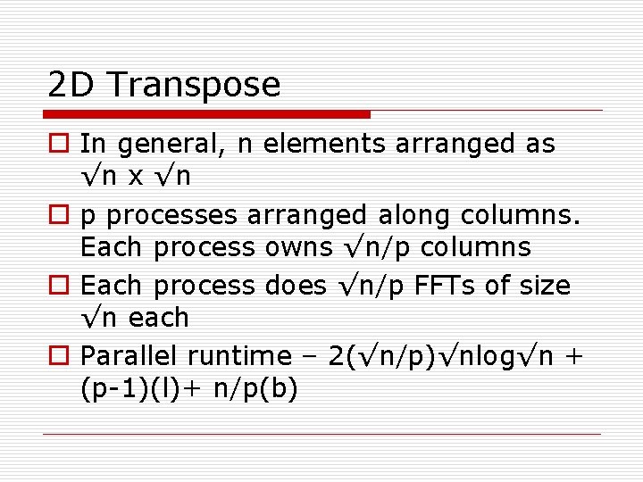
2 D Transpose o In general, n elements arranged as √n x √n o p processes arranged along columns. Each process owns √n/p columns o Each process does √n/p FFTs of size √n each o Parallel runtime – 2(√n/p)√nlog√n + (p-1)(l)+ n/p(b)

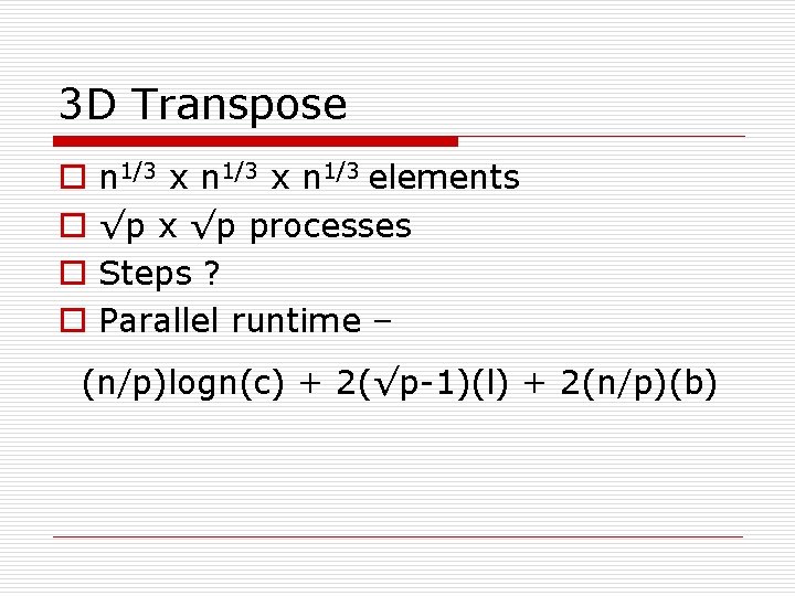
3 D Transpose o o n 1/3 x n 1/3 elements √p x √p processes Steps ? Parallel runtime – (n/p)logn(c) + 2(√p-1)(l) + 2(n/p)(b)

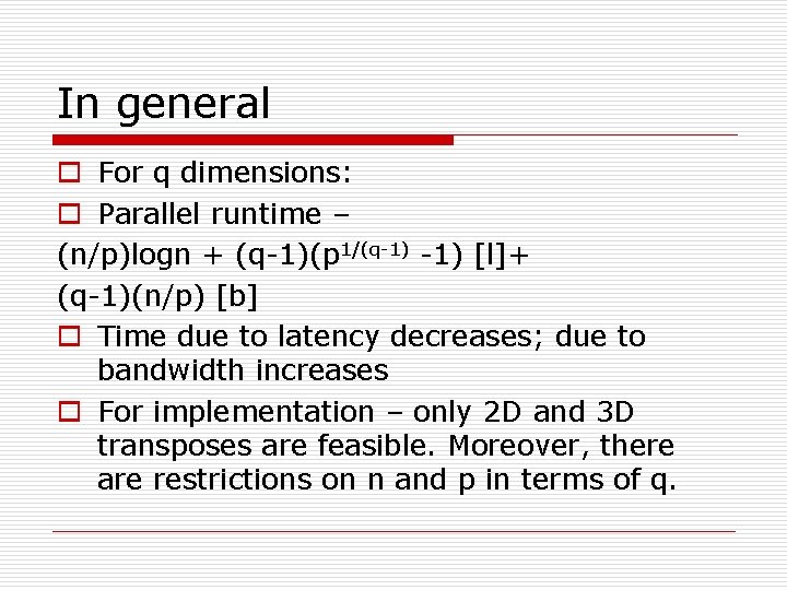
In general o For q dimensions: o Parallel runtime – (n/p)logn + (q-1)(p 1/(q-1) [l]+ (q-1)(n/p) [b] o Time due to latency decreases; due to bandwidth increases o For implementation – only 2 D and 3 D transposes are feasible. Moreover, there are restrictions on n and p in terms of q.

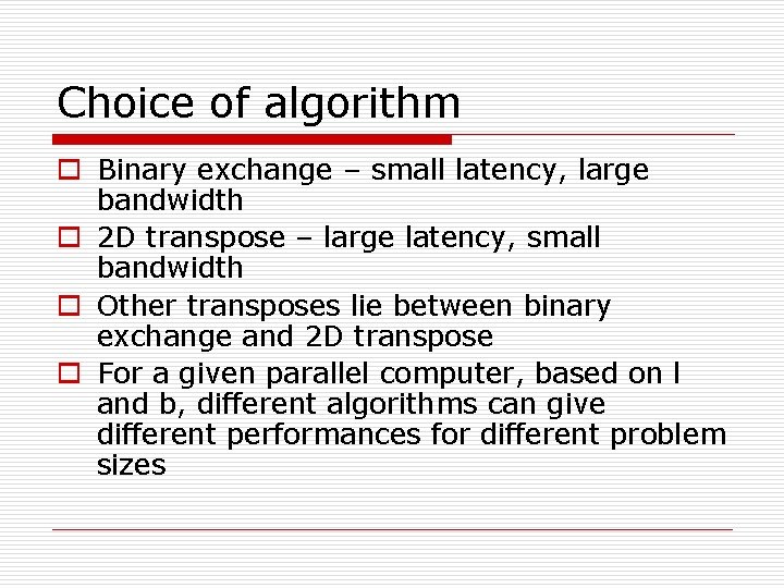
Choice of algorithm o Binary exchange – small latency, large bandwidth o 2 D transpose – large latency, small bandwidth o Other transposes lie between binary exchange and 2 D transpose o For a given parallel computer, based on l and b, different algorithms can give different performances for different problem sizes