Image Transforms and Image Enhancement in Frequency Domain

Image Transforms and Image Enhancement in Frequency Domain Lecture 5, Feb 25 th, 2008 Lexing Xie EE 4830 Digital Image Processing http: //www. ee. columbia. edu/~xlx/ee 4830/ thanks to G&W website, Mani Thomas, Min Wu and Wade Trappe for slide materials

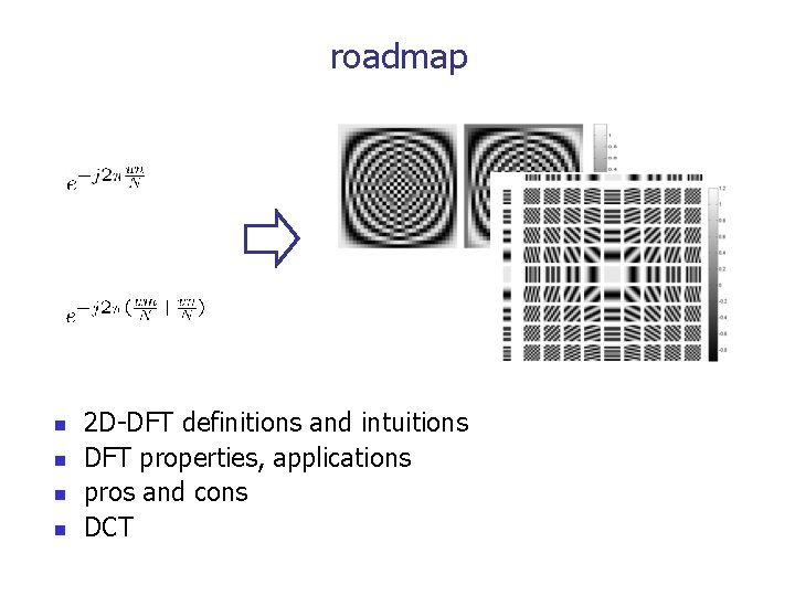
roadmap n n 2 D-DFT definitions and intuitions DFT properties, applications pros and cons DCT

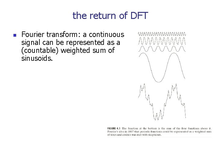
the return of DFT n Fourier transform: a continuous signal can be represented as a (countable) weighted sum of sinusoids.

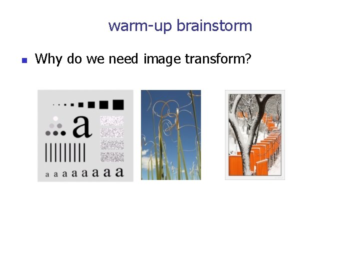
warm-up brainstorm n Why do we need image transform?

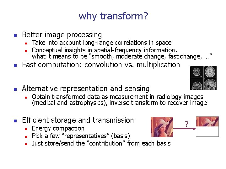
why transform? n Better image processing n n Take into account long-range correlations in space Conceptual insights in spatial-frequency information. what it means to be “smooth, moderate change, fast change, …” n Fast computation: convolution vs. multiplication n Alternative representation and sensing n n Obtain transformed data as measurement in radiology images (medical and astrophysics), inverse transform to recover image Efficient storage and transmission n Energy compaction Pick a few “representatives” (basis) Just store/send the “contribution” from each basis ?

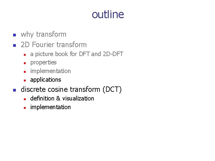
outline n n why transform 2 D Fourier transform n n n a picture book for DFT and 2 D-DFT properties implementation applications discrete cosine transform (DCT) n n definition & visualization Implementation next lecture: transform of all flavors, unitary transform, KLT, others …

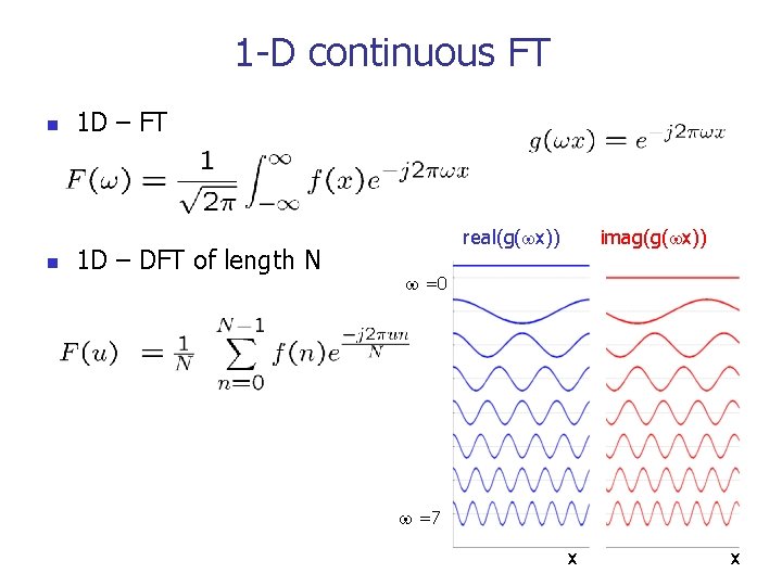
1 -D continuous FT n n 1 D – FT 1 D – DFT of length N real(g( x)) imag(g( x)) =0 =7 x x

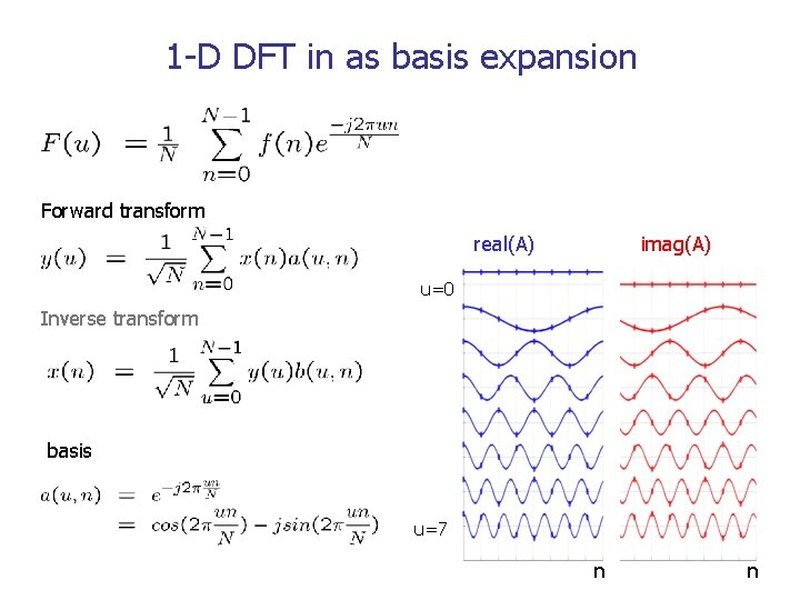
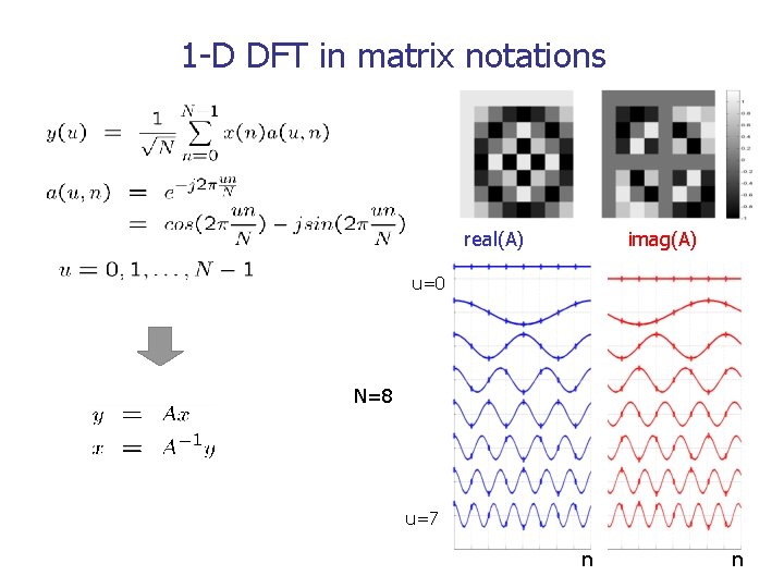
1 -D DFT in as basis expansion Forward transform real(A) imag(A) u=0 Inverse transform basis u=7 n n

1 -D DFT in matrix notations real(A) imag(A) u=0 N=8 u=7 n n

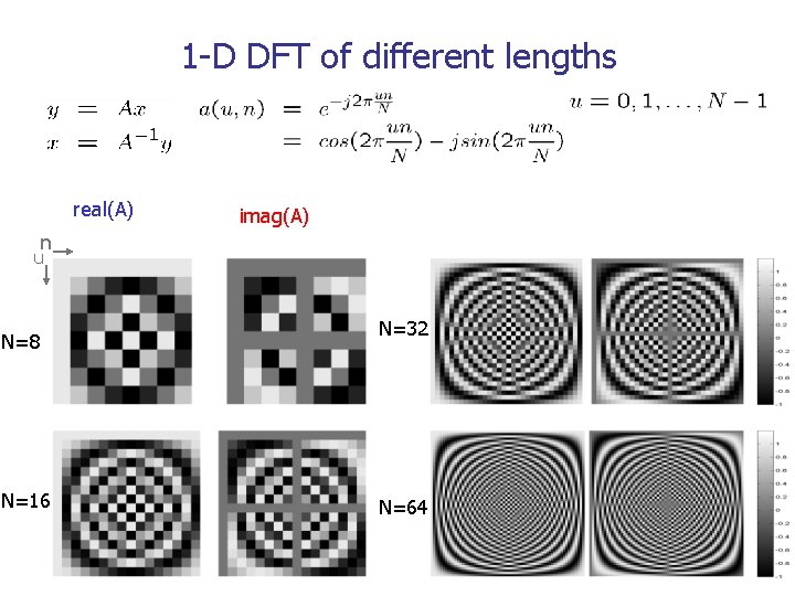
1 -D DFT of different lengths real(A) imag(A) n u N=8 N=16 N=32 N=64

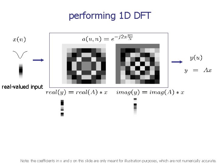
performing 1 D DFT real-valued input Note: the coefficients in x and y on this slide are only meant for illustration purposes, which are not numerically accurate.

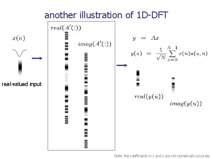
another illustration of 1 D-DFT real-valued input Note: the coefficients in x and y are not numerically accurate

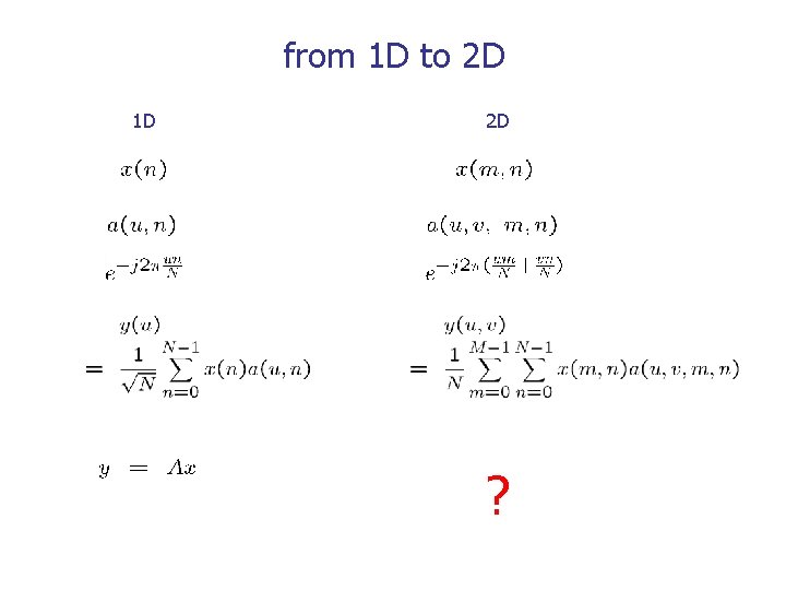
from 1 D to 2 D 1 D 2 D ?

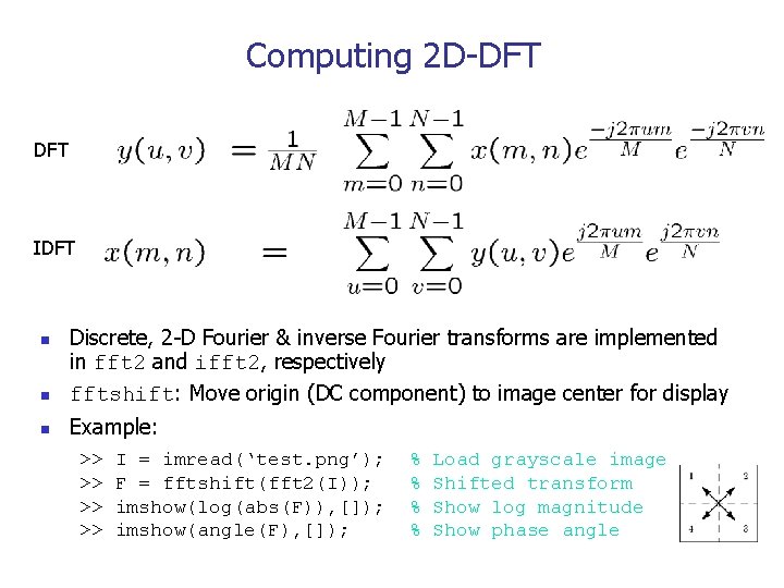
Computing 2 D-DFT IDFT n Discrete, 2 -D Fourier & inverse Fourier transforms are implemented in fft 2 and ifft 2, respectively fftshift: Move origin (DC component) to image center for display n Example: n >> >> I = imread(‘test. png’); F = fftshift(fft 2(I)); imshow(log(abs(F)), []); imshow(angle(F), []); % % Load grayscale image Shifted transform Show log magnitude Show phase angle

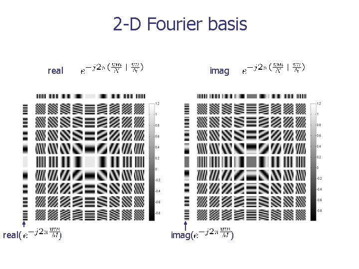
2 -D Fourier basis real( ) imag( )

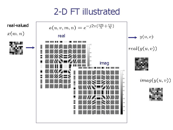
2 -D FT illustrated real-valued real imag

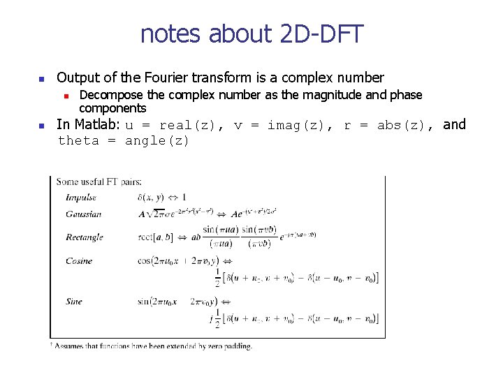
notes about 2 D-DFT n Output of the Fourier transform is a complex number n n Decompose the complex number as the magnitude and phase components In Matlab: u = real(z), v = imag(z), r = abs(z), and theta = angle(z)

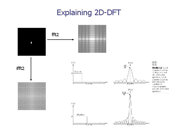
Explaining 2 D-DFT fft 2 ifft 2

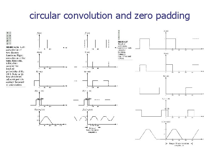
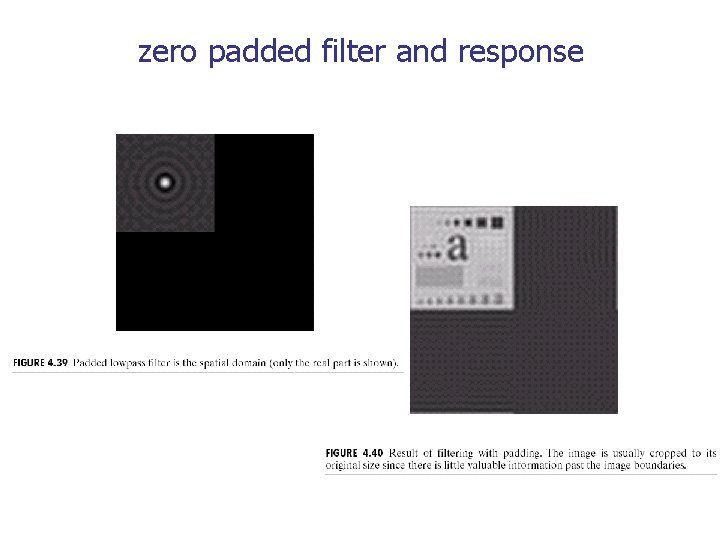
circular convolution and zero padding

zero padded filter and response

zero padded filter and response

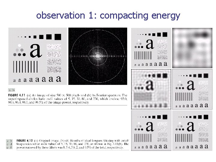
observation 1: compacting energy

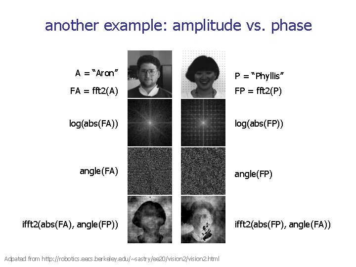
observation 2: amplitude vs. phase n n Amplitude: relative prominence of sinusoids Phase: relative displacement of sinusoids

another example: amplitude vs. phase A = “Aron” P = “Phyllis” FA = fft 2(A) FP = fft 2(P) log(abs(FA)) log(abs(FP)) angle(FA) ifft 2(abs(FA), angle(FP)) Adpated from http: //robotics. eecs. berkeley. edu/~sastry/ee 20/vision 2. html angle(FP) ifft 2(abs(FP), angle(FA))

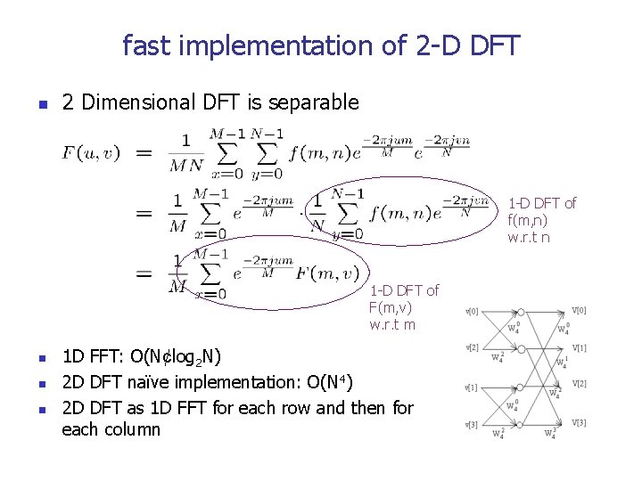
fast implementation of 2 -D DFT n 2 Dimensional DFT is separable 1 -D DFT of f(m, n) w. r. t n 1 -D DFT of F(m, v) w. r. t m n n n 1 D FFT: O(N¢log 2 N) 2 D DFT naïve implementation: O(N 4) 2 D DFT as 1 D FFT for each row and then for each column

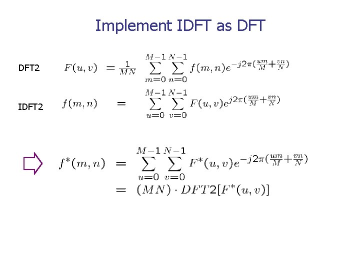
Implement IDFT as DFT 2 IDFT 2

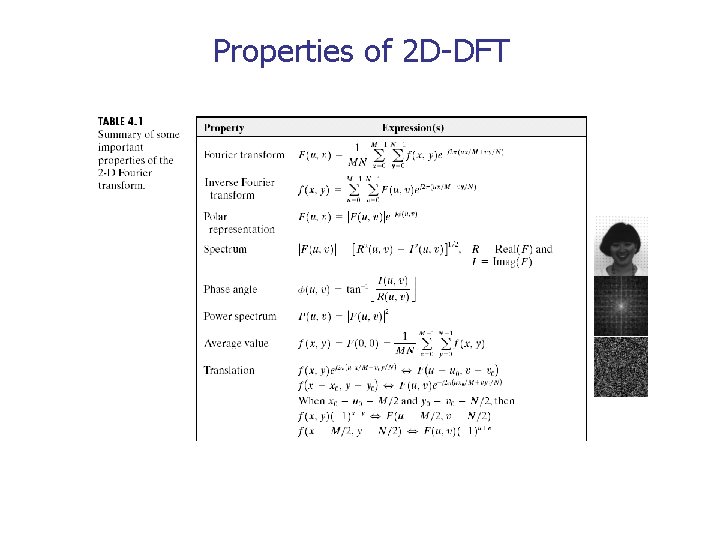
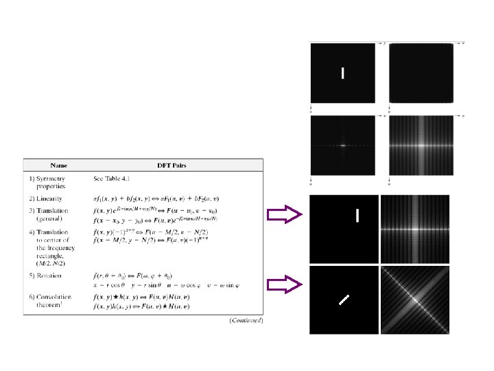
Properties of 2 D-DFT

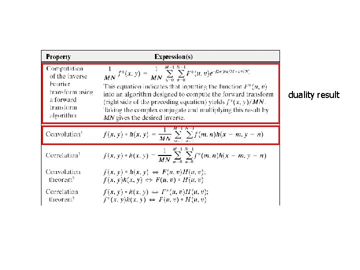
duality result

outline n n why transform 2 D Fourier transform n n n a picture book for DFT and 2 D-DFT properties implementation applications discrete cosine transform (DCT) n n definition & visualization implementation

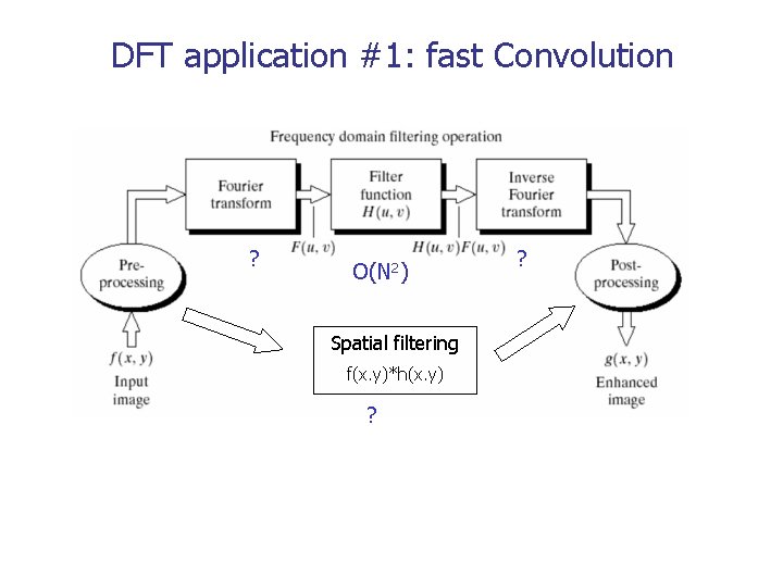
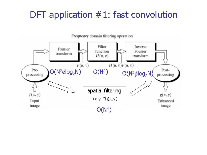
DFT application #1: fast Convolution ? O(N 2) Spatial filtering f(x. y)*h(x. y) ? ?

DFT application #1: fast convolution O(N 2¢log 2 N) O(N 2) Spatial filtering f(x. y)*h(x. y) O(N 4) O(N 2¢log 2 N)

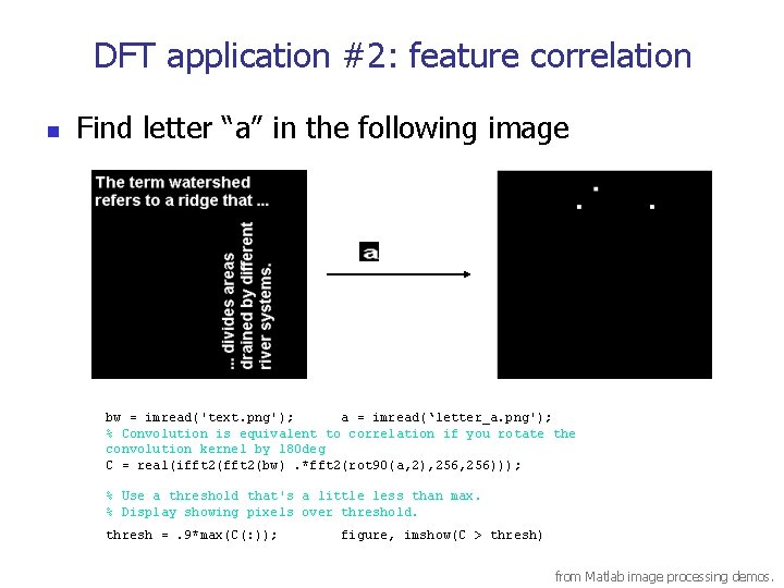
DFT application #2: feature correlation n Find letter “a” in the following image bw = imread('text. png'); a = imread(‘letter_a. png'); % Convolution is equivalent to correlation if you rotate the convolution kernel by 180 deg C = real(ifft 2(bw). *fft 2(rot 90(a, 2), 256))); % Use a threshold that's a little less than max. % Display showing pixels over threshold. thresh =. 9*max(C(: )); figure, imshow(C > thresh) from Matlab image processing demos.

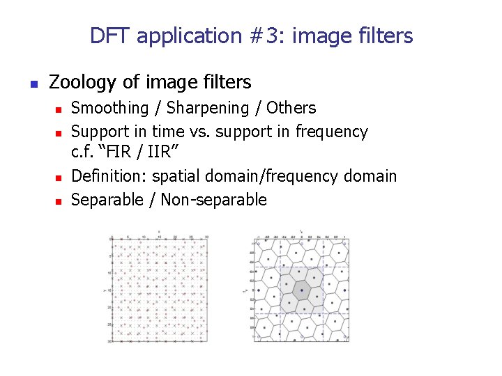
DFT application #3: image filters n Zoology of image filters n n Smoothing / Sharpening / Others Support in time vs. support in frequency c. f. “FIR / IIR” Definition: spatial domain/frequency domain Separable / Non-separable

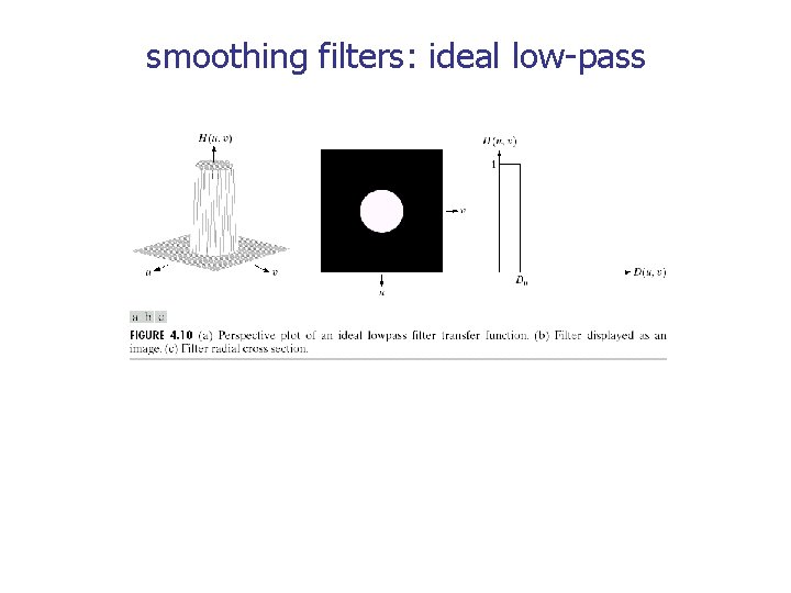
smoothing filters: ideal low-pass

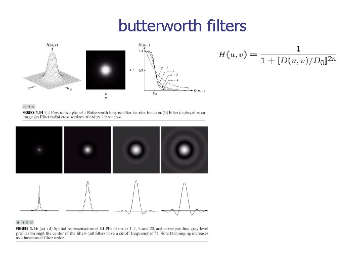
butterworth filters

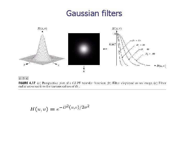
Gaussian filters

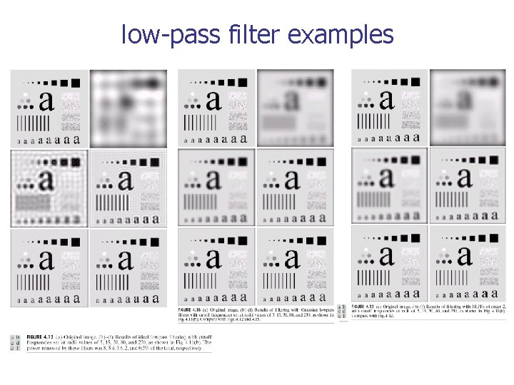
low-pass filter examples

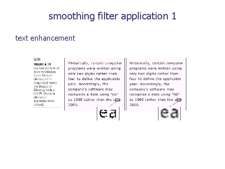
smoothing filter application 1 text enhancement

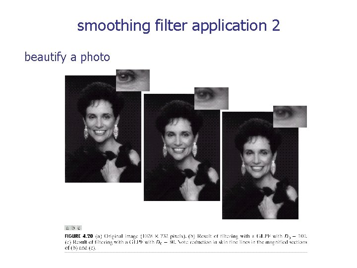
smoothing filter application 2 beautify a photo

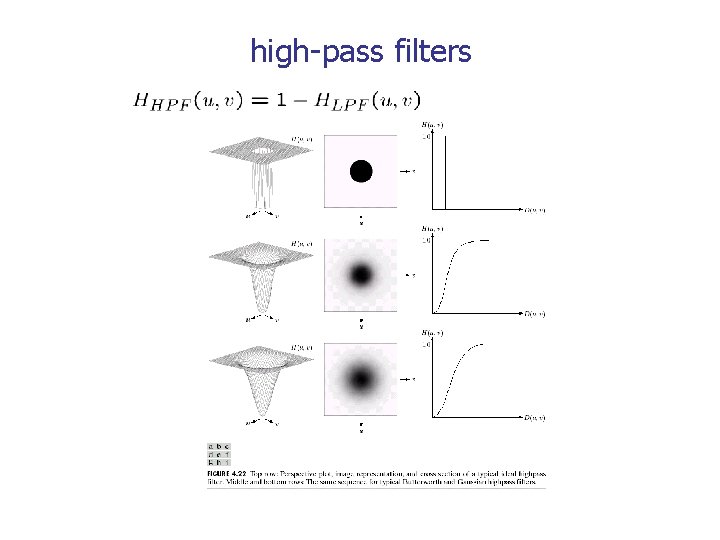
high-pass filters

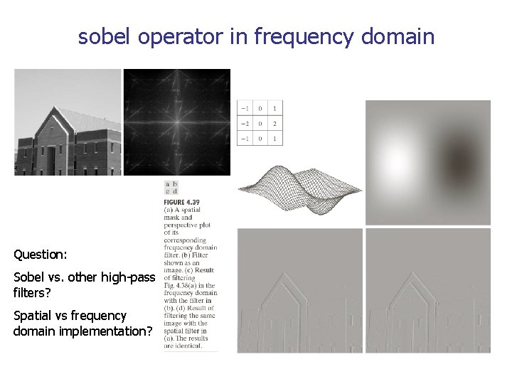
sobel operator in frequency domain Question: Sobel vs. other high-pass filters? Spatial vs frequency domain implementation?

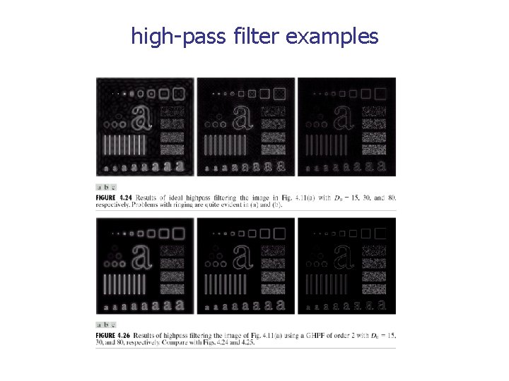
high-pass filter examples

outline n n why transform 2 D Fourier transform n n n a picture book for DFT and 2 D-DFT properties implementation applications in enhancement, correlation discrete cosine transform (DCT) n n definition & visualization implementation

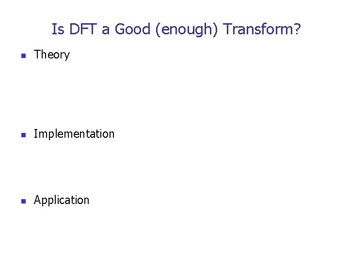
Is DFT a Good (enough) Transform? n Theory n Implementation n Application

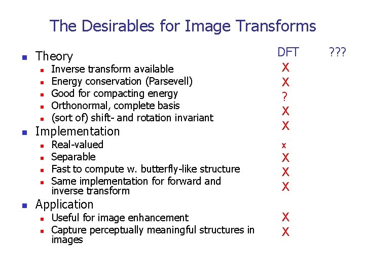
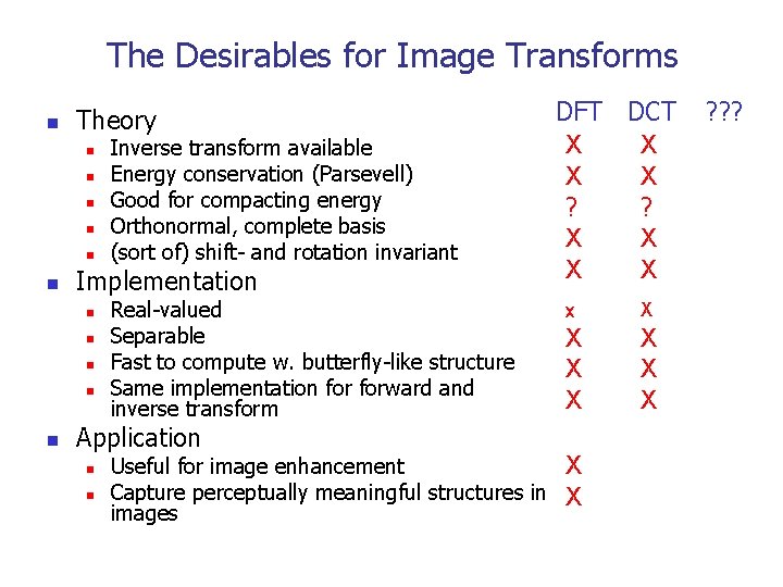
The Desirables for Image Transforms n Theory n n n Implementation n n Inverse transform available Energy conservation (Parsevell) Good for compacting energy Orthonormal, complete basis (sort of) shift- and rotation invariant Real-valued Separable Fast to compute w. butterfly-like structure Same implementation forward and inverse transform Application n n Useful for image enhancement Capture perceptually meaningful structures in images DFT X X ? X X x X X X ? ? ?

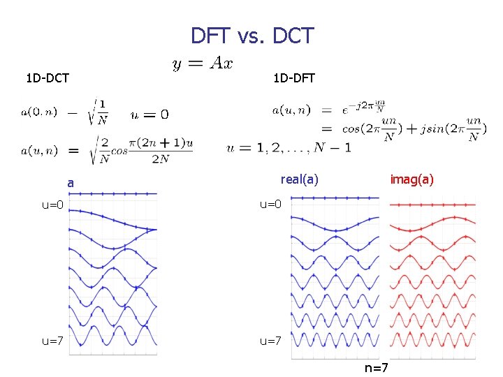
DFT vs. DCT 1 D-DFT real(a) a u=0 u=7 imag(a) n=7

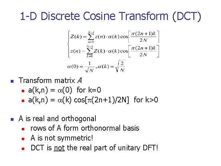
1 -D Discrete Cosine Transform (DCT) n n Transform matrix A n a(k, n) = (0) for k=0 n a(k, n) = (k) cos[ (2 n+1)/2 N] for k>0 A is real and orthogonal n rows of A form orthonormal basis n A is not symmetric! n DCT is not the real part of unitary DFT!

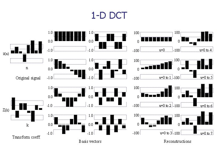
1 -D DCT z(n) n Original signal Z(k) k Transform coeff. 1. 0 100 100 0. 0 0 0 -100 u=0 to 1 -100 1. 0 100 0. 0 0 0 -100 u=0 to 2 -100 1. 0 100 0. 0 0 0 -100 u=0 to 3 -100 Basis vectors u=0 -100 Reconstructions u=0 to 4 u=0 to 5 u=0 to 6 u=0 to 7

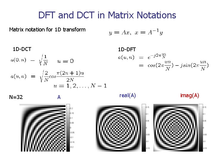
DFT and DCT in Matrix Notations Matrix notation for 1 D transform 1 D-DCT N=32 1 D-DFT A real(A) imag(A)

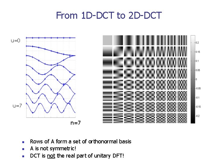
From 1 D-DCT to 2 D-DCT u=0 u=7 n n n Rows of A form a set of orthonormal basis A is not symmetric! DCT is not the real part of unitary DFT!

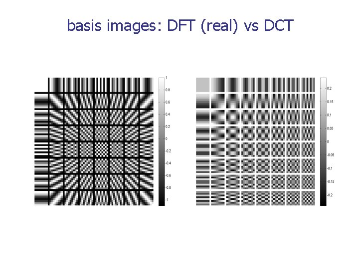
basis images: DFT (real) vs DCT

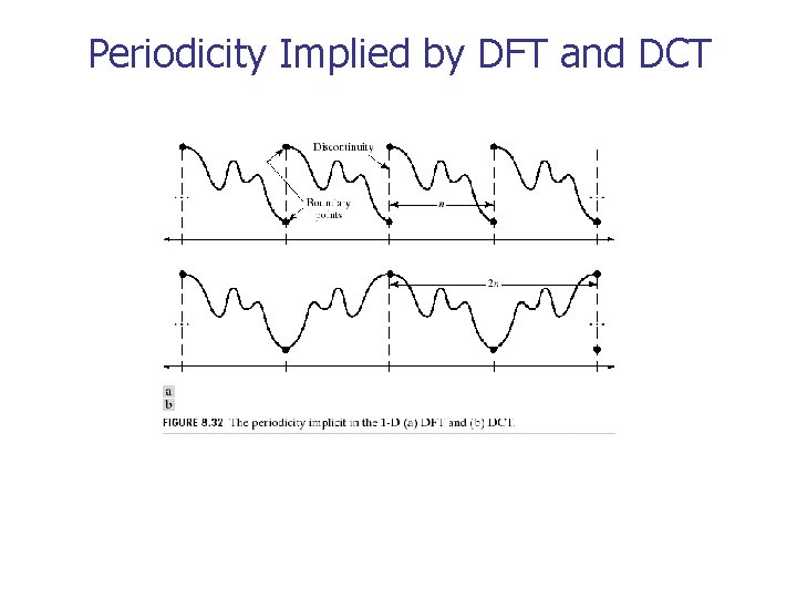
Periodicity Implied by DFT and DCT

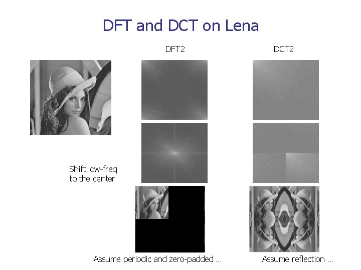
DFT and DCT on Lena DFT 2 DCT 2 Shift low-freq to the center Assume periodic and zero-padded … Assume reflection …

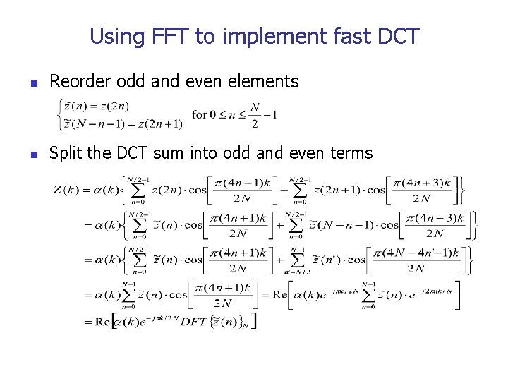
Using FFT to implement fast DCT n Reorder odd and even elements n Split the DCT sum into odd and even terms

The Desirables for Image Transforms n Theory n n n Implementation n n Inverse transform available Energy conservation (Parsevell) Good for compacting energy Orthonormal, complete basis (sort of) shift- and rotation invariant Real-valued Separable Fast to compute w. butterfly-like structure Same implementation forward and inverse transform Application n n Useful for image enhancement Capture perceptually meaningful structures in images DFT DCT X X ? ? X X x X X X X X ? ? ?

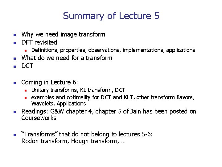
Summary of Lecture 5 n n Why we need image transform DFT revisited n Definitions, properties, observations, implementations, applications n What do we need for a transform DCT n Coming in Lecture 6: n n n Unitary transforms, KL transform, DCT examples and optimality for DCT and KLT, other transform flavors, Wavelets, Applications Readings: G&W chapter 4, chapter 5 of Jain has been posted on Courseworks “Transforms” that do not belong to lectures 5 -6: Rodon transform, Hough transform, …