CH 4 Image Enhancement in the Frequency Domain

CH 4. Image Enhancement in the Frequency Domain

Domain Change

Content This chapter is concerned primarily with helping the reader develop a basic understanding of the Fourier transform and the frequency domain, and how they apply to image enhancement. 4. 1 Background 4. 2 Introduction to the Fourier Transform and the Freq. Domain 4. 3 Smoothing Frequency-Domain Filters 4. 4 Sharpening Frequency-Domain Filters 4. 5 Homomorphic Filtering 4. 6 Implementation

4. 1 Background • Any function that periodically repeats itself can be expressed as the sum of sines and/or cosines of different frequencies, each multiplied by a different coefficient (Fourier series). • Even functions that are not periodic (but whose area under the curve is finite) can be expressed as the integral of sines and/or cosines multiplied by a weighting function (Fourier transform). • The advent of digital computation and the “discovery” of fast Fourier Transform (FFT) algorithm in the late 1950 s revolutionized the field of signal processing.

• The frequency domain refers to the plane of the two dimensional discrete Fourier transform of an image. • The purpose of the Fourier transform is to represent a signal as a linear combination of sinusoidal signals of various frequencies.

4. 2 Introduction to the Fourier Transform and the Frequency Domain • The one-dimensional Fourier transform and its inverse – Fourier transform (continuous case) – Inverse Fourier transform: • The two-dimensional Fourier transform and its inverse – Fourier transform (continuous case) – Inverse Fourier transform:

4. 2. 1 The one-dimensional Fourier transform and its inverse (discrete time case) ◦ Fourier transform (DFT) ◦ Inverse Fourier transform (IDFT) The 1/M multiplier in front of the Fourier transform sometimes is placed in the front of the inverse instead. Other times both equations are multiplied by

Since and the fact then discrete Fourier transform can be redefined ◦ Frequency domain: the domain (values of u) over which the values of F(u) range; because u determines the frequency of the components of the transform. ◦ Frequency component: each of the M terms of F(u).

Mathematical Prism

F(u) can be expressed in polar coordinates: ◦ R(u): the real part of F(u) ◦ I(u): the imaginary part of F(u) Power spectrum:

One-Dimensional Fourier Transform Examples Please note the relationship between the value of K and the height of the spectrum and the number of zeros in the frequency domain.

4. 2. 2 The two-dimensional Fourier transform and its inverse (discrete time case) ◦ Fourier transform (DFT) ◦ Inverse Fourier transform (IDFT) u, v : the transform or frequency variables x, y : the spatial or image variables

The Fourier spectrum, phase angle, and power spectrum of the two-dimensional Fourier transform as follows: ◦ R(u, v): the real part of F(u, v) ◦ I(u, v): the imaginary part of F(u, v)

Some properties of Fourier transform:

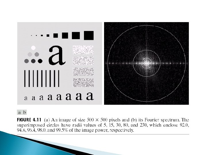
Consider the relationship between the separation of zeros in u- or vdirection and the width or height of white block of source image.

4. 2. 3 Filtering in the Frequency Domain - Frequency is directly related to rate of change. -The frequency of fast varying components in an image is higher than slowly varying components.

Basics of Filtering in the Frequency Domain Including multiplication the input/output image by (-1)x+y. What is zero-phase-shift filter?

Some Basic Filters and Their Functions Multiply all values of F(u, v) by the filter function (notch filter): ◦ All this filter would do is set F(0, 0) to zero (force the average value of an image to zero) and leave all other frequency components of the Fourier transform untouched and make prominent edges stand out.

Some Basic Filters and Their Functions Lowpass filter Circular symmetry Highpass filter

Some Basic Filters and Their Functions Low pass filters: eliminate the gray-level detail and keep the general gray-level appearance. (blurring the image) High pass filters: have less gray-level variations in smooth areas and emphasized transitional (e. g. , edge and noise) gray-level detail. (sharpening images)

4. 2. 4 Correspondence between Filtering in the Spatial and Frequency Domain Convolution theorem: ◦ The discrete convolution of two functions f(x, y) and h(x, y) of size M N is defined as The process of implementation: 1) Flipping one function about the origin; 2) Shifting that function with respect to the other by changing the values of (x, y); 3) Computing a sum of products over all values of m and n, for each displacement.

–Let F(u, v) and H(u, v) denote the Fourier transforms of f(x, y) and h(x, y), then Eq. (4. 2 -31) Eq. (4. 2 -32) • an impulse function of strength A, located at coordinates (x 0, y 0): and is defined by : The shifting property of impulse function where : a unit impulse located at the origin • The Fourier transform of a unit impulse at the origin (Eq 4. 2 -35) :

Let , then the convolution (Eq. (4. 2 -36)) Combine Eqs. (4. 2 -35) (4. 2 -36) with Eq. (4. 2 -31), we obtain: That is to say, the response of impulse input is the transfer function of filter.

The distinction and links between spatial and frequency filtering l l l If the size of spatial and frequency filters is same, then the computation burden in spatial domain is larger than in frequency domain; However, whenever possible, it makes more sense to filter in the spatial domain using small filter masks. Filtering in frequency is more intuitive. We can specify filters in the frequency, take their inverse transform, and the use the resulting filter in spatial domain as a guide for constructing smaller spatial filter masks.

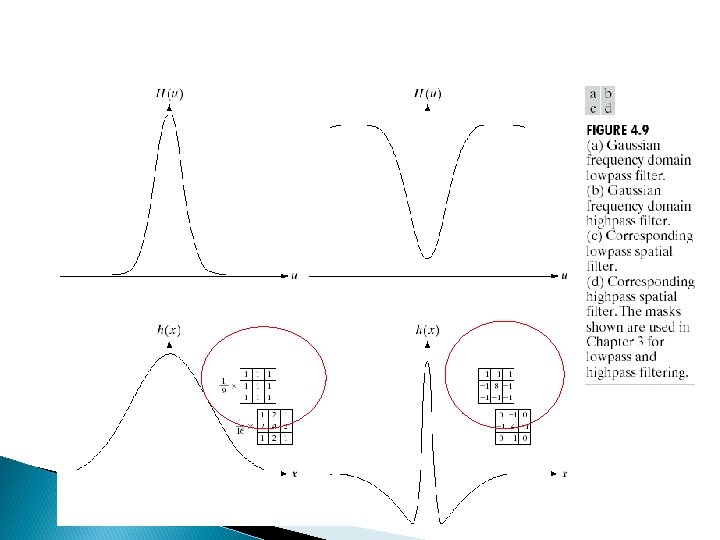
Two reasons that filters based on Gaussian functions are of particular importance: 1) their shapes are easily specified; 2) both the forward and inverse Fourier transforms of a Gaussian are real Gaussian function. Let H(u) denote a frequency domain, Gaussian filter function given the equation where: - the standard deviation of the Gaussian curve. The corresponding filter in the spatial domain is

The corresponding filter in the spatial domain is We can note that the value of this types of filter has both negative and positive values. Once the values turn negative, they never turn positive again. Filtering in frequency domain is usually used for the guides to design the filter masks in the spatial domain.

4. 3 Smoothing Frequency-Domain Filters The basic model for filtering in the frequency domain where F(u, v): the Fourier transform of the image to be smoothed H(u, v): a filter transfer function Smoothing is fundamentally a lowpass operation in the frequency domain. There are several standard forms of lowpass filters (LPF). ◦ Ideal lowpass filter ◦ Butterworth lowpass filter ◦ Gaussian lowpass filter

Ideal Lowpass Filters (ILPFs) The simplest lowpass filter is a filter that “cuts off” all high-frequency components of the Fourier transform that are at a distance greater than a specified distance D 0 from the origin of the transform. The transfer function of an ideal lowpass filter where D(u, v) : the distance from point (u, v) to the center of the frequency rectangle (M/2, N/2)

Cut-off Frequency ILPF is a type of “nonphysical” filters and can’t be realized with electronic components and is not very practical.

The blurring and ringing phenomena can be seen, in which ringing behavior is characteristic of ideal filters.

Another example of ILPF Figure 4. 13 (a) A frequency-domain ILPF of radius 5. (b) Corresponding spatial filter. (c) Five impulses in the spatial domain, simulating the values of five pixels. (d) Convolution of (b) and (c) in the spatial domain. Notation: the radius of center component and the number of circles per unit distance from the origin are inversely proportional to the value of the cutoff frequency. diagonal scan line of (d) frequency spatial

Butterworth Lowpass Filters (BLPFs) with order n Note the relationship between order n and smoothing The BLPF may be viewed as a transition between ILPF and GLPF, BLPF of order 2 is a good compromise between effective lowpass filtering and acceptable ringing characteristics.

Butterworth Lowpass Filters (BLPFs) n=2 D 0=5, 15, 30, 80, and 230

Butterworth Lowpass Filters (BLPFs) Spatial Representation n=1 n=2 n=5 n=20

Gaussian Lowpass Filters (FLPFs)

Gaussian Lowpass Filters (FLPFs) D 0=5, 15, 30, 80, and 230

Additional Examples of Lowpass Filtering Character recognition in machine perception: join the broken character segments with a Gaussian lowpass filter with D 0=80.

Application in “cosmetic processing” and produce a smoother, softer-looking result from a sharp original.

Gaussian lowpass filter for reducing the horizontal sensor scan lines and simplifying the detection of features like the interface boundaries.

Summary 4. 1 Background - Fourier series, Fourier transform 4. 2 Introduction to the Fourier Transform and the Freq. Domain - DFT and its inverse, property of freq. domain, Basic of filtering, Noch filter, Lowpass, High pass, Correspondence between filtering in spatial domain and freq. domain 4. 3 Smoothing Frequency-Domain Filters - ILPF, Ringing, BLPF, GLPF