Chapter 3 Image Enhancement Image Enhancement The principal

Chapter 3 Image Enhancement

Image Enhancement The principal objective of enhancement is to process an image so that the result is more suitable than the original image for a specific application The specific application may determine approaches or techniques for image enhancement Image enhancement approaches fall into two broad categories Spatial domain methods Frequency domain methods

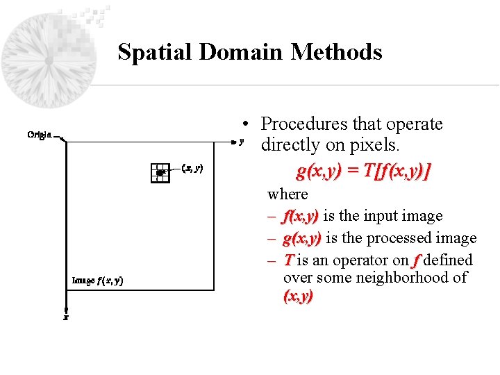
Spatial Domain Methods • Procedures that operate directly on pixels. g(x, y) = T[f(x, y)] where – f(x, y) is the input image – g(x, y) is the processed image – T is an operator on f defined over some neighborhood of (x, y)

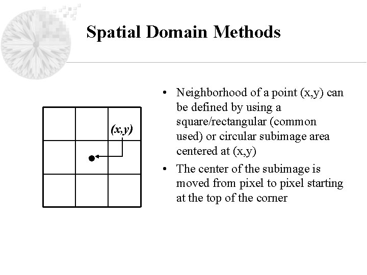
Spatial Domain Methods (x, y) • • Neighborhood of a point (x, y) can be defined by using a square/rectangular (common used) or circular subimage area centered at (x, y) • The center of the subimage is moved from pixel to pixel starting at the top of the corner

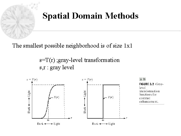
Spatial Domain Methods The smallest possible neighborhood is of size 1 x 1 s=T(r) ; gray-level transformation s, r : gray level

Gray Level Transformations

Image Negatives Image in the range [0, L-1] It is useful in displaying medical images

Image Negatives

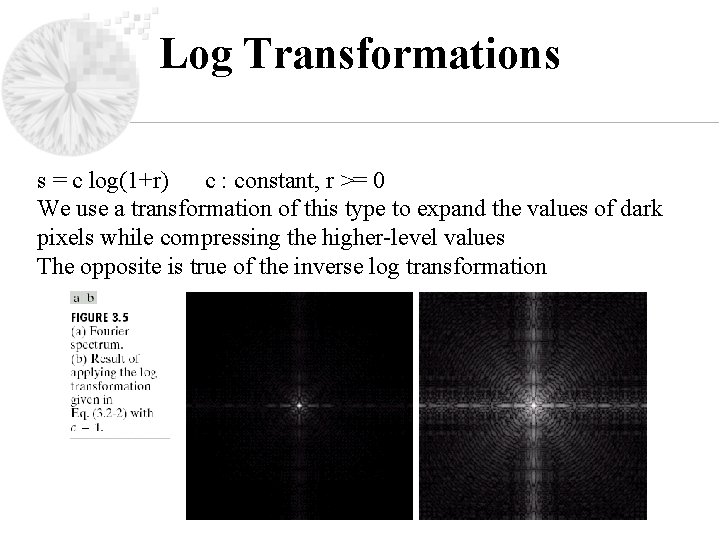
Log Transformations s = c log(1+r) c : constant, r >= 0 We use a transformation of this type to expand the values of dark pixels while compressing the higher-level values The opposite is true of the inverse log transformation

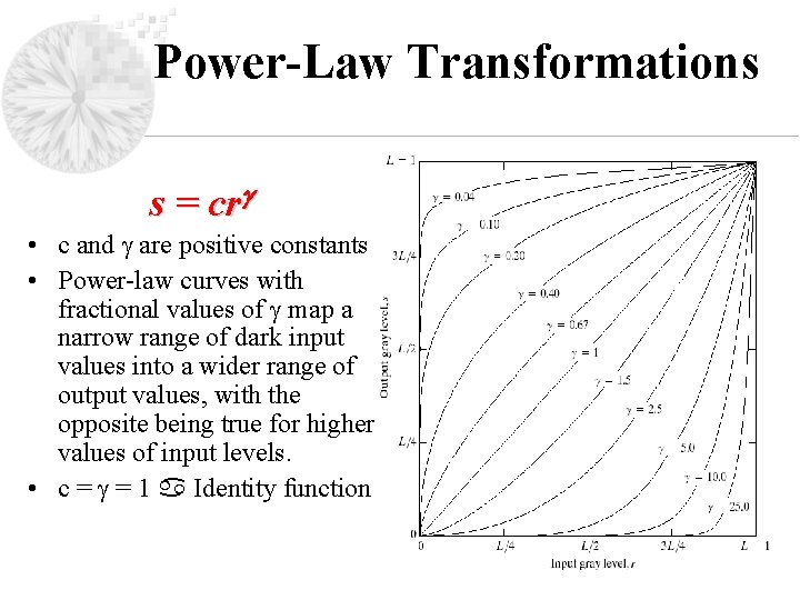
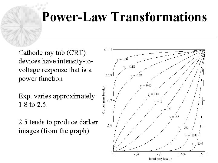
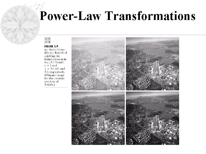
Power-Law Transformations s = cr • c and are positive constants • Power-law curves with fractional values of map a narrow range of dark input values into a wider range of output values, with the opposite being true for higher values of input levels. • c = = 1 Identity function

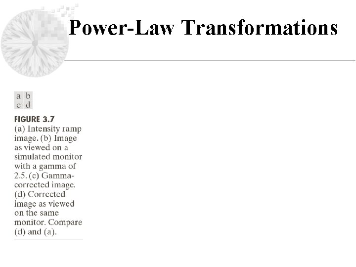
Power-Law Transformations Cathode ray tub (CRT) devices have intensity-tovoltage response that is a power function Exp. varies approximately 1. 8 to 2. 5 tends to produce darker images (from the graph)

Power-Law Transformations

Power-Law Transformations

Power-Law Transformations

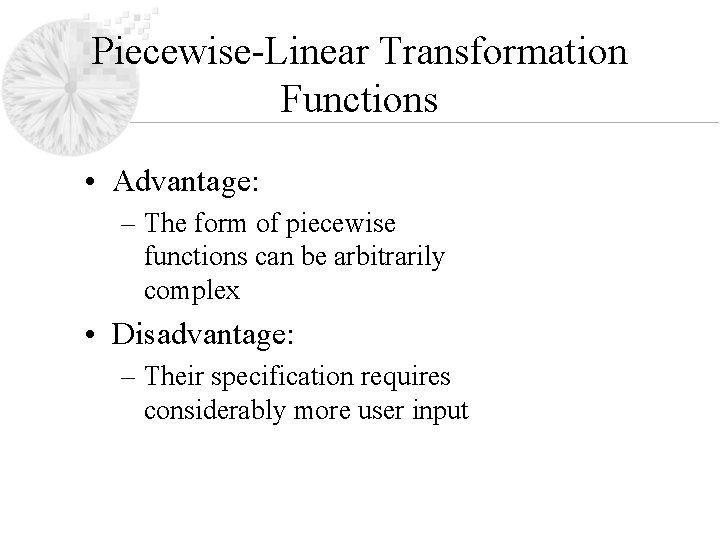
Piecewise-Linear Transformation Functions • Advantage: – The form of piecewise functions can be arbitrarily complex • Disadvantage: – Their specification requires considerably more user input

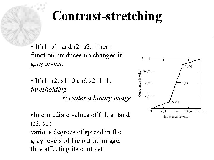
Contrast-stretching • If r 1=s 1 and r 2=s 2, linear function produces no changes in gray levels. • If r 1=r 2, s 1=0 and s 2=L-1, thresholding • creates a binary image • Intermediate values of (r 1, s 1)and (r 2, s 2) various degrees of spread in the gray levels of the output image, thus affecting its contrast.

Contrast-stretching • increase the dynamic range of the gray levels in the image • (b) a low-contrast image • (c) result of contrast stretching: (r 1, s 1) = (rmin, 0) and (r 2, s 2) = (rmax, L-1) • (d) result of thresholding

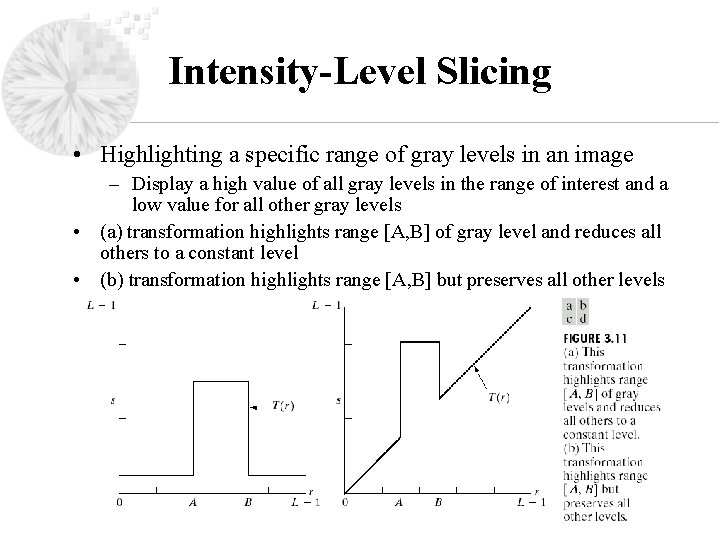
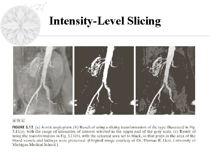
Intensity-Level Slicing • Highlighting a specific range of gray levels in an image – Display a high value of all gray levels in the range of interest and a low value for all other gray levels • (a) transformation highlights range [A, B] of gray level and reduces all others to a constant level • (b) transformation highlights range [A, B] but preserves all other levels

Intensity-Level Slicing

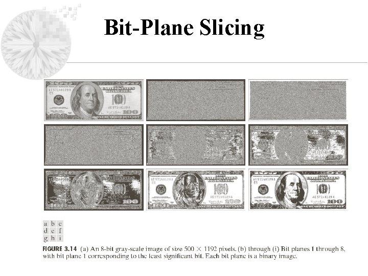
Bit-Plane Slicing Highlighting the contribution made to total image appearance by specific bits

Bit-Plane Slicing

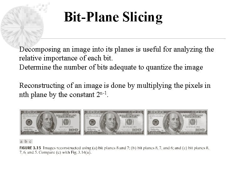
Bit-Plane Slicing Decomposing an image into its planes is useful for analyzing the relative importance of each bit. Determine the number of bits adequate to quantize the image Reconstructing of an image is done by multiplying the pixels in nth plane by the constant 2 n-1.

Histogram Processing • Histogram of a digital image with gray levels in the range [0, L-1] is a discrete function • h(rk) = nk • Where – rk : the kth gray level – nk : the number of pixels in the image having gray level rk – h(rk) : histogram of a digital image with gray levels rk - p(rk) = nk/MN , k=0, 1, …, L-1 - p(rk) is an estimate of the probability of occurrence of gray level k

Histogram Processing

Histogram Processing

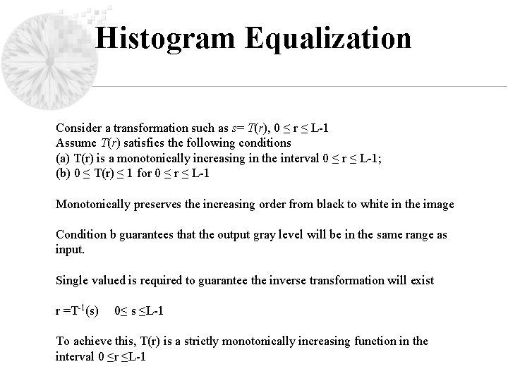
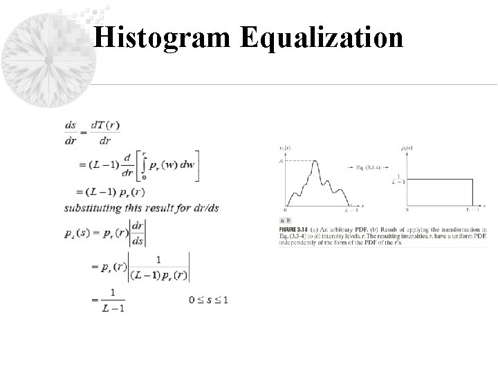
Histogram Equalization Consider a transformation such as s= T(r), 0 ≤ r ≤ L-1 Assume T(r) satisfies the following conditions (a) T(r) is a monotonically increasing in the interval 0 ≤ r ≤ L-1; (b) 0 ≤ T(r) ≤ 1 for 0 ≤ r ≤ L-1 Monotonically preserves the increasing order from black to white in the image Condition b guarantees that the output gray level will be in the same range as input. Single valued is required to guarantee the inverse transformation will exist r =T-1(s) 0≤ s ≤L-1 To achieve this, T(r) is a strictly monotonically increasing function in the interval 0 ≤r ≤L-1

Histogram Equalization

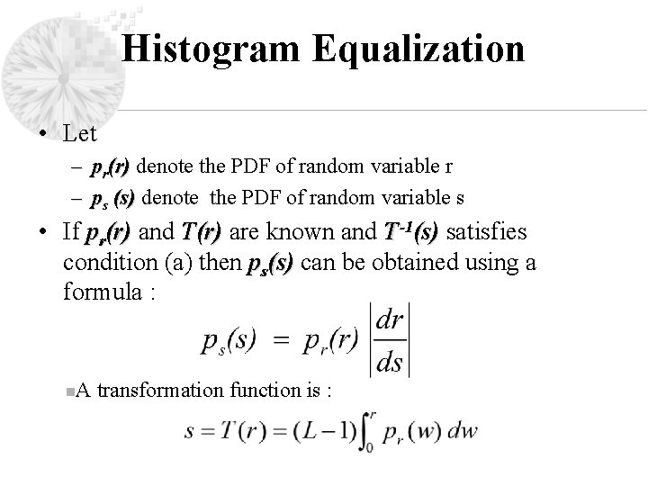
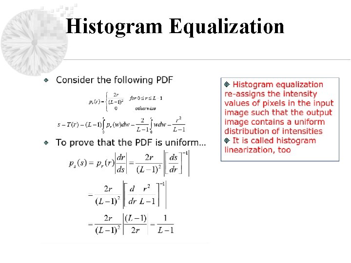
Histogram Equalization • Let – pr(r) denote the PDF of random variable r – ps (s) denote the PDF of random variable s • If pr(r) and T(r) are known and T-1(s) satisfies condition (a) then ps(s) can be obtained using a formula : n A transformation function is :

Histogram Equalization

Histogram Equalization

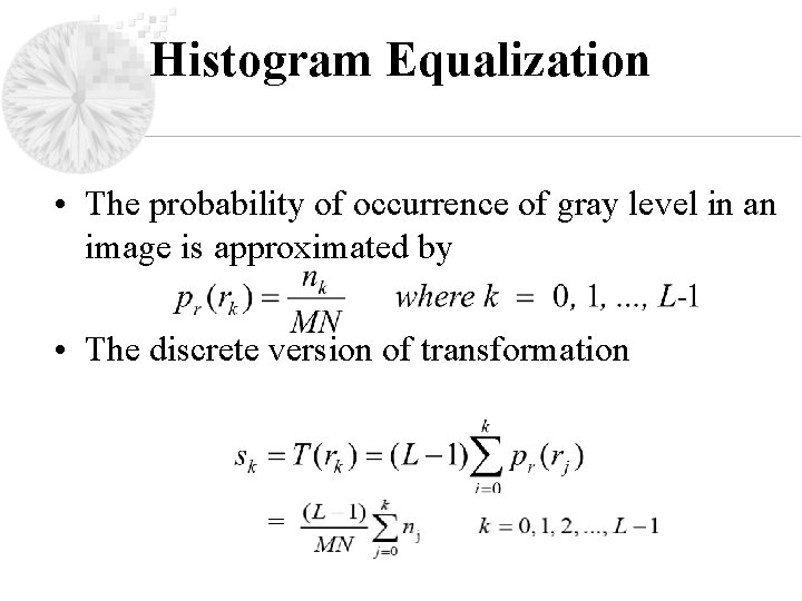
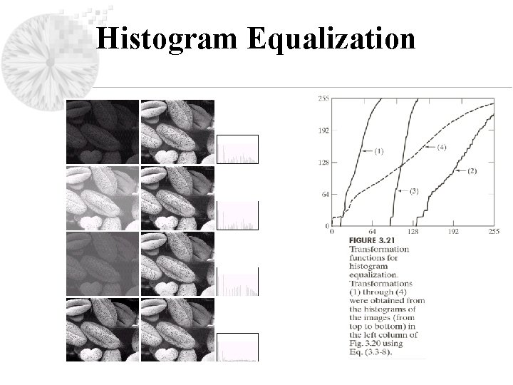
Histogram Equalization • The probability of occurrence of gray level in an image is approximated by • The discrete version of transformation =

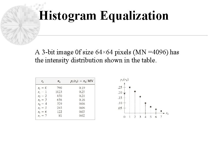
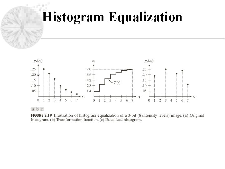
Histogram Equalization A 3 -bit image 0 f size 64× 64 pixels (MN =4096) has the intensity distribution shown in the table.

Histogram Equalization

Histogram Equalization

Histogram Equalization

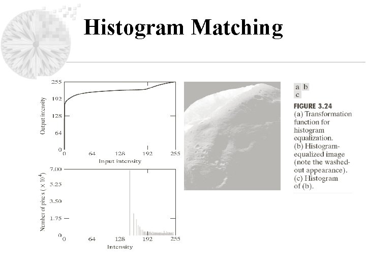
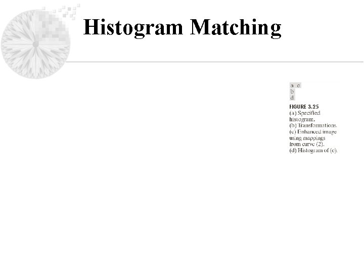
Histogram Matching histogram equalization automatically determines a transformation function that seeks to produce an output image that has a uniform histogram Some applications in which attempting to enhancement based on a uniform histogram is not the best approach The method used to generate a processed image that has a specified histogram is called histogram matching or histogram specification.

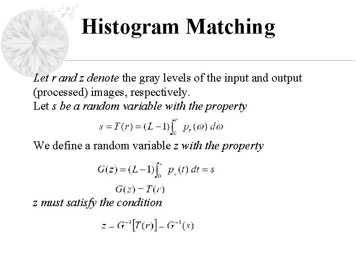
Histogram Matching Let r and z denote the gray levels of the input and output (processed) images, respectively. Let s be a random variable with the property We define a random variable z with the property z must satisfy the condition

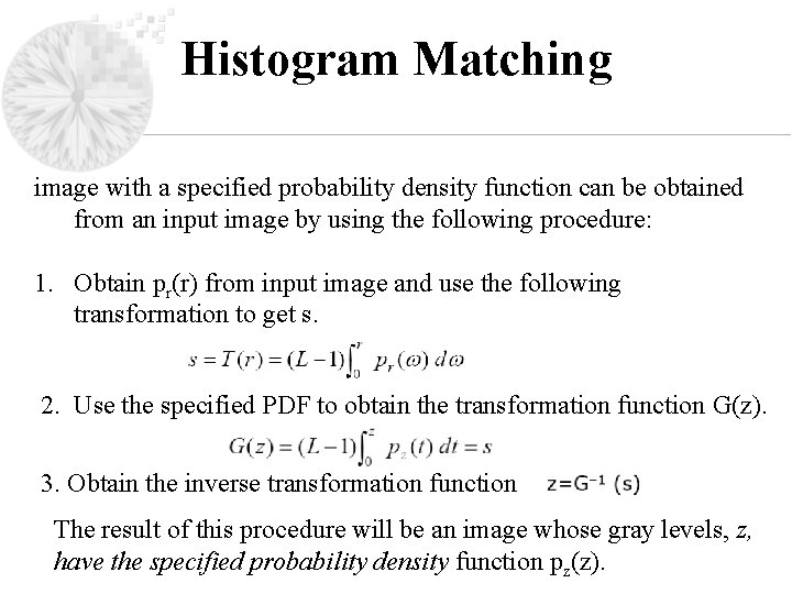
Histogram Matching image with a specified probability density function can be obtained from an input image by using the following procedure: 1. Obtain pr(r) from input image and use the following transformation to get s. 2. Use the specified PDF to obtain the transformation function G(z). 3. Obtain the inverse transformation function The result of this procedure will be an image whose gray levels, z, have the specified probability density function pz(z).

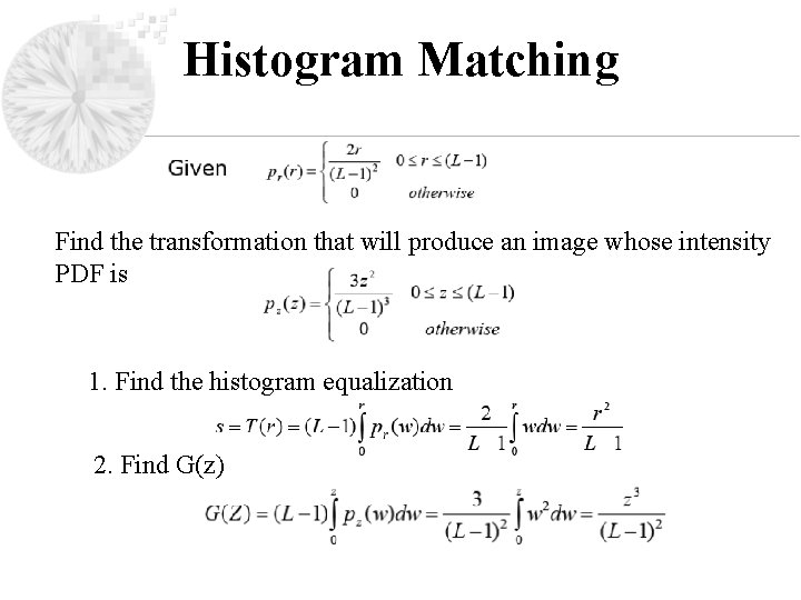
Histogram Matching Find the transformation that will produce an image whose intensity PDF is 1. Find the histogram equalization 2. Find G(z)

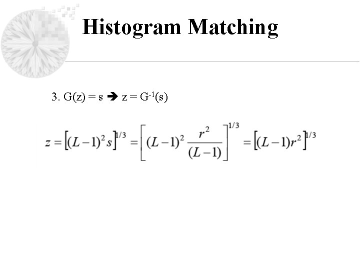
Histogram Matching 3. G(z) = s z = G-1(s)

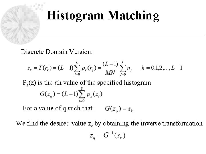
Histogram Matching Discrete Domain Version: Pz(z) is the ith value of the specified histogram For a value of q such that : We find the desired value zq by obtaining the inverse transformation

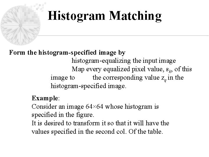
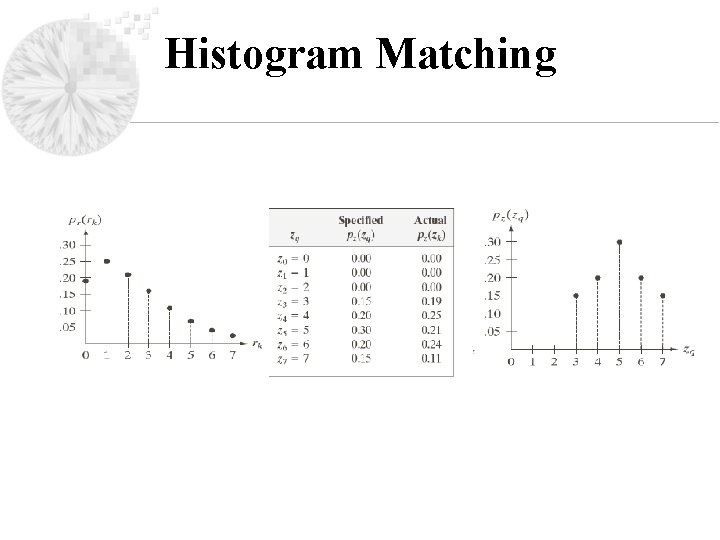
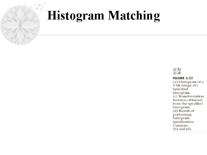
Histogram Matching Form the histogram-specified image by histogram-equalizing the input image Map every equalized pixel value, sk, of this image to the corresponding value zq in the histogram-specified image. Example: Consider an image 64× 64 whose histogram is specified in the figure. It is desired to transform it so that it will have the values specified in the second col. Of the table.

Histogram Matching

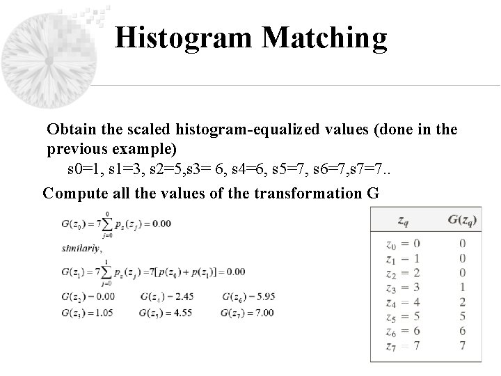
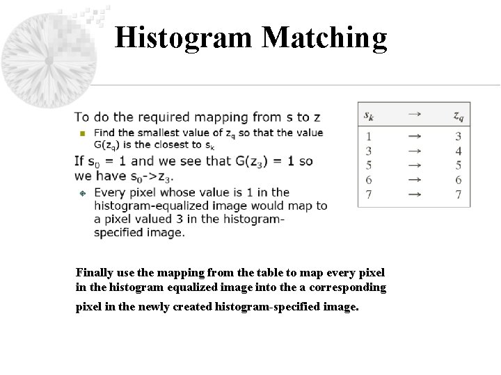
Histogram Matching Obtain the scaled histogram-equalized values (done in the previous example) s 0=1, s 1=3, s 2=5, s 3= 6, s 4=6, s 5=7, s 6=7, s 7=7. . Compute all the values of the transformation G

Histogram Matching Finally use the mapping from the table to map every pixel in the histogram equalized image into the a corresponding pixel in the newly created histogram-specified image.

Histogram Matching

Histogram Matching

Histogram Matching

Histogram Matching

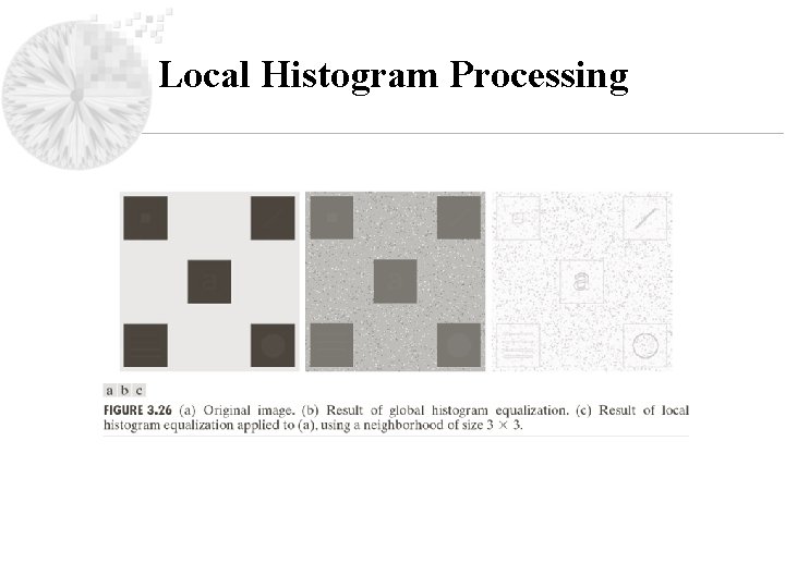
Local Histogram Processing • Histogram processing methods are global processing, in the sense that pixels are modified by a transformation function based on the gray-level content of an entire image. • Sometimes, we may need to enhance details over small areas in an image, which is called a local enhancement.

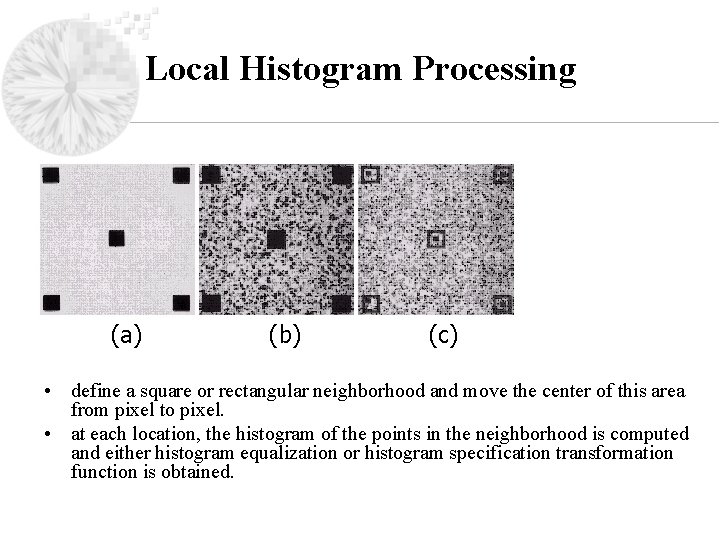
Local Histogram Processing (a) (b) (c) • define a square or rectangular neighborhood and move the center of this area from pixel to pixel. • at each location, the histogram of the points in the neighborhood is computed and either histogram equalization or histogram specification transformation function is obtained.

Local Histogram Processing

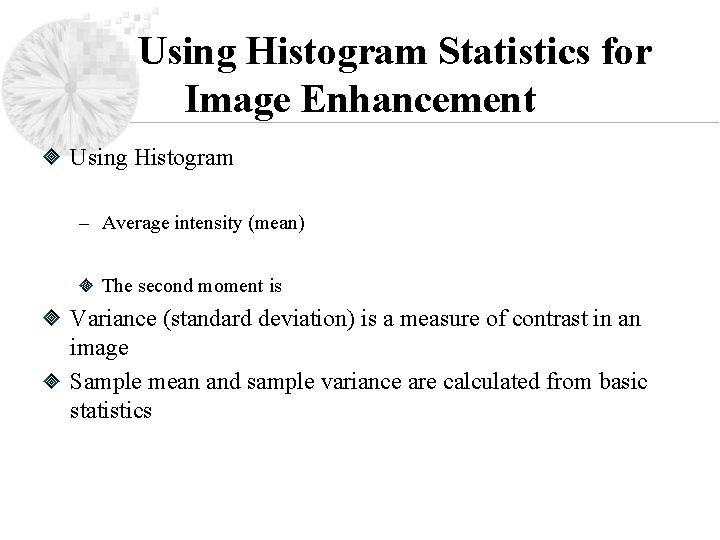
Using Histogram Statistics for Image Enhancement Using Histogram – Average intensity (mean) The second moment is Variance (standard deviation) is a measure of contrast in an image Sample mean and sample variance are calculated from basic statistics

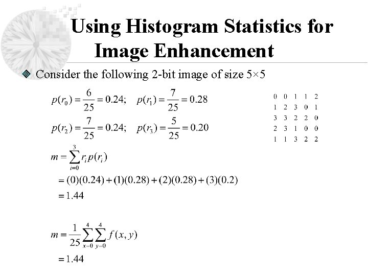
Using Histogram Statistics for Image Enhancement Consider the following 2 -bit image of size 5× 5

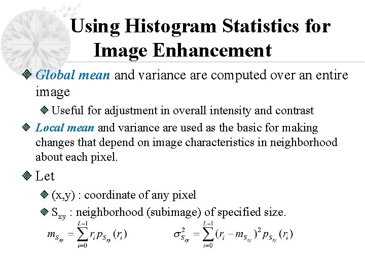
Using Histogram Statistics for Image Enhancement Global mean and variance are computed over an entire image Useful for adjustment in overall intensity and contrast Local mean and variance are used as the basic for making changes that depend on image characteristics in neighborhood about each pixel. Let (x, y) : coordinate of any pixel Sxy : neighborhood (subimage) of specified size.

Using Histogram Statistics for Image Enhancement

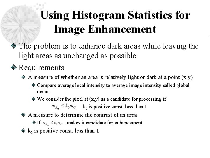
Using Histogram Statistics for Image Enhancement The problem is to enhance dark areas while leaving the light areas as unchanged as possible Requirements A measure of whether an area is relatively light or dark at a point (x, y) Compare average local intensity to average image intensity called global mean. We consider the pixel at (x, y) as a candidate for processing if k 0 is positive const. less than 1 A measure to determine the contrast of an area If makes it candidate for enhancement k 2 is positive const. less than 1

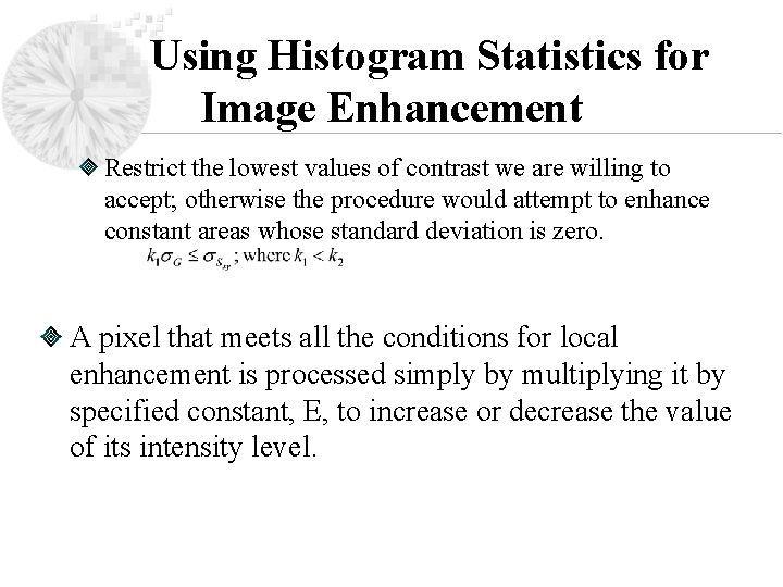
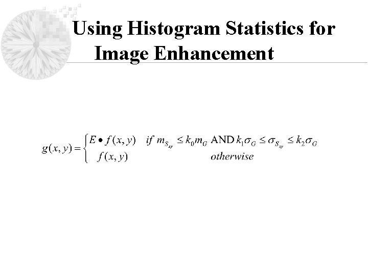
Using Histogram Statistics for Image Enhancement Restrict the lowest values of contrast we are willing to accept; otherwise the procedure would attempt to enhance constant areas whose standard deviation is zero. A pixel that meets all the conditions for local enhancement is processed simply by multiplying it by specified constant, E, to increase or decrease the value of its intensity level.

Using Histogram Statistics for Image Enhancement

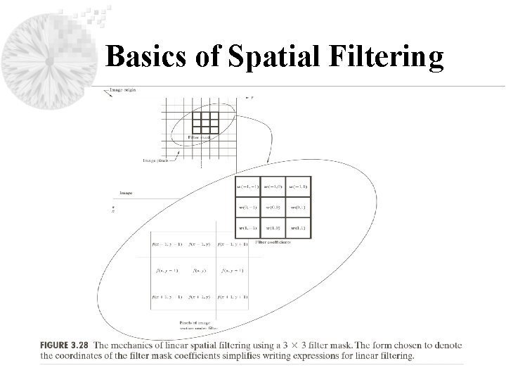
Basics of Spatial Filtering Spatial filter consists of Neighborhood (small rectangle) Predefined operation Performed on the image pixels encompassed by the neighborhood New pixel is created coordinates equal to the coordinates of the center of the neighborhood value is the result of the operation Linear if operation is linear

Basics of Spatial Filtering

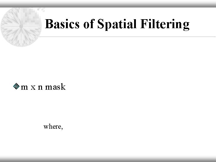
Basics of Spatial Filtering m x n mask where,

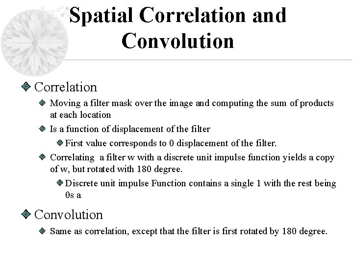
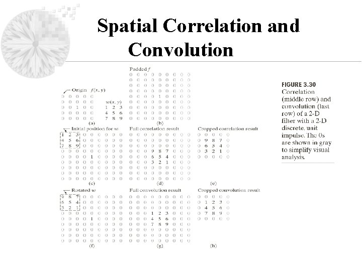
Spatial Correlation and Convolution Correlation Moving a filter mask over the image and computing the sum of products at each location Is a function of displacement of the filter First value corresponds to 0 displacement of the filter. Correlating a filter w with a discrete unit impulse function yields a copy of w, but rotated with 180 degree. Discrete unit impulse Function contains a single 1 with the rest being 0 s a Convolution Same as correlation, except that the filter is first rotated by 180 degree.

Spatial Correlation and Convolution

Spatial Correlation and Convolution

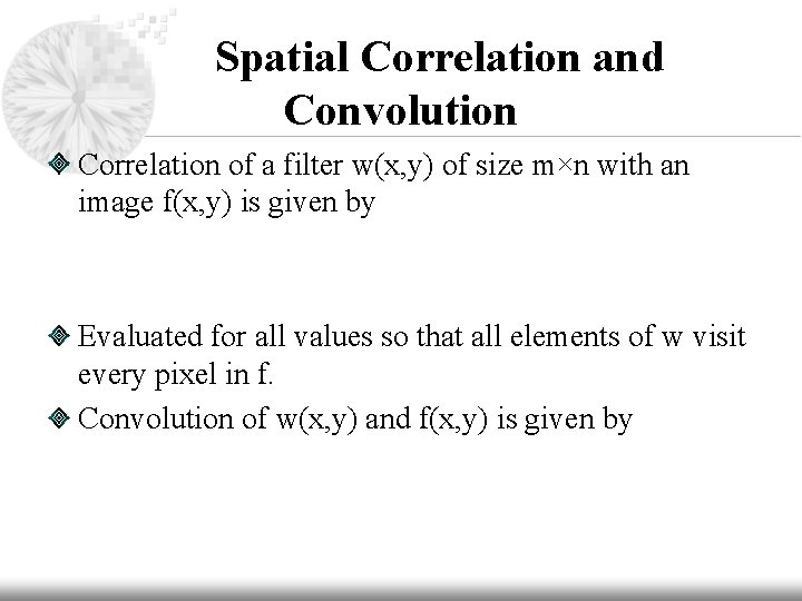
Spatial Correlation and Convolution Correlation of a filter w(x, y) of size m×n with an image f(x, y) is given by Evaluated for all values so that all elements of w visit every pixel in f. Convolution of w(x, y) and f(x, y) is given by

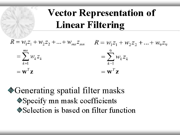
Vector Representation of Linear Filtering Generating spatial filter masks Specify mn mask coefficients Selection is based on filter function

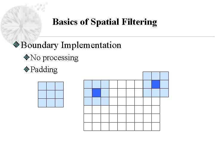
Basics of Spatial Filtering Boundary Implementation No processing Padding

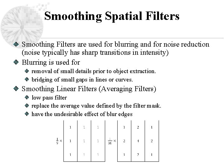
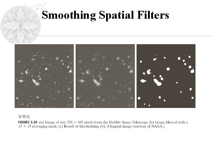
Smoothing Spatial Filters Smoothing Filters are used for blurring and for noise reduction (noise typically has sharp transitions in intensity) Blurring is used for removal of small details prior to object extraction. bridging of small gaps in lines or curves. Smoothing Linear Filters (Averaging Filters) low pass filter replace the average value defined by the filter mask. have the undesirable effect of blur edges

Smoothing Spatial Filters weighted average Pixels have different importance The pixel at the center is multiplied by a higher value The other pixels are inversely weighted as a function of distance The weight like this attempts to reduce the blurring effect in the smoothing process Sum of all weights is 16 (easy for computer implementation because it is a power of 2) Other values of weight could accomplish the same general objectives

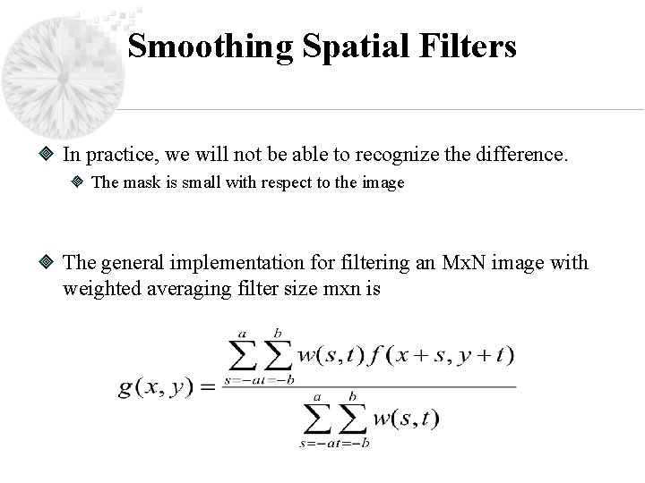
Smoothing Spatial Filters In practice, we will not be able to recognize the difference. The mask is small with respect to the image The general implementation for filtering an Mx. N image with weighted averaging filter size mxn is

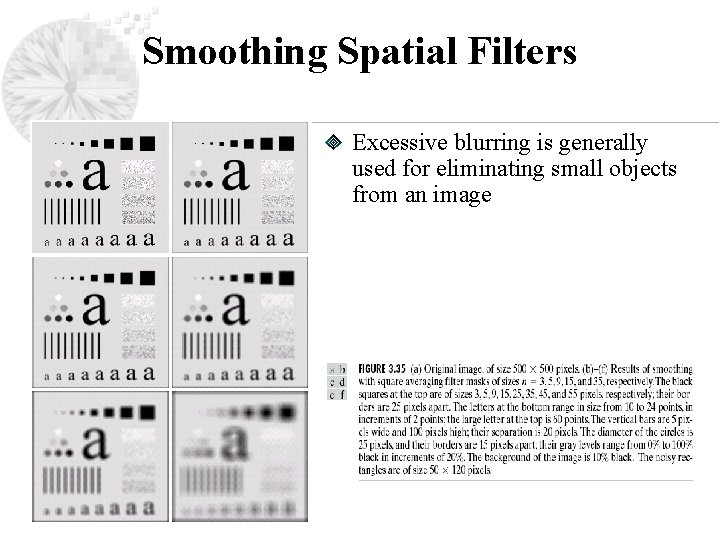
Smoothing Spatial Filters Excessive blurring is generally used for eliminating small objects from an image

Smoothing Spatial Filters

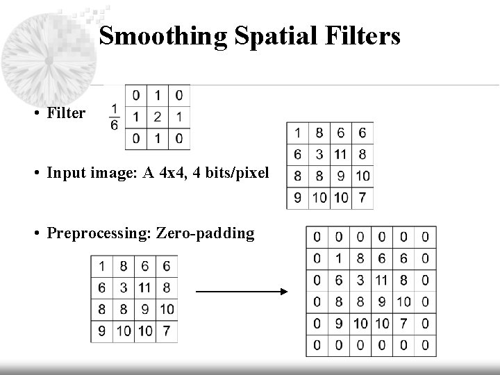
Smoothing Spatial Filters • Filter • Input image: A 4 x 4, 4 bits/pixel • Preprocessing: Zero-padding

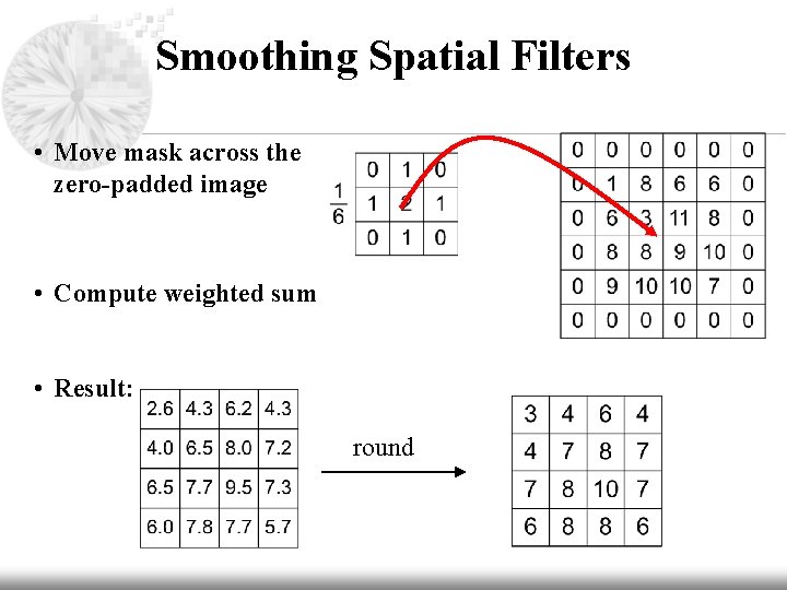
Smoothing Spatial Filters • Move mask across the zero-padded image • Compute weighted sum • Result: round

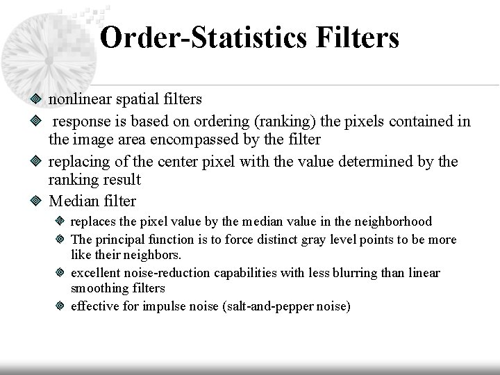
Order-Statistics Filters nonlinear spatial filters response is based on ordering (ranking) the pixels contained in the image area encompassed by the filter replacing of the center pixel with the value determined by the ranking result Median filter replaces the pixel value by the median value in the neighborhood The principal function is to force distinct gray level points to be more like their neighbors. excellent noise-reduction capabilities with less blurring than linear smoothing filters effective for impulse noise (salt-and-pepper noise)

Median Filter

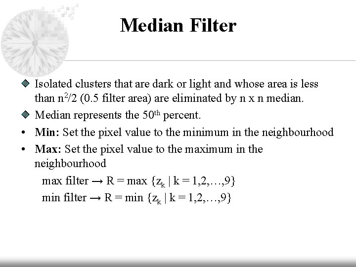
Median Filter Isolated clusters that are dark or light and whose area is less than n 2/2 (0. 5 filter area) are eliminated by n x n median. Median represents the 50 th percent. • Min: Set the pixel value to the minimum in the neighbourhood • Max: Set the pixel value to the maximum in the neighbourhood max filter → R = max {zk | k = 1, 2, …, 9} min filter → R = min {zk | k = 1, 2, …, 9}

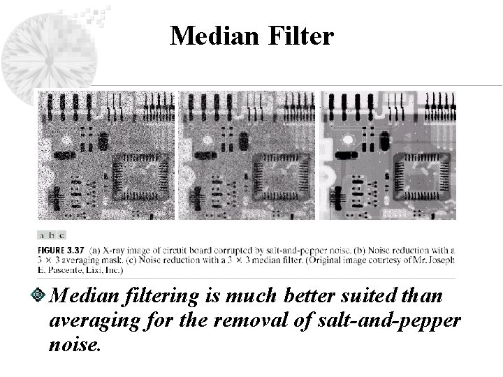
Median Filter Median filtering is much better suited than averaging for the removal of salt-and-pepper noise.

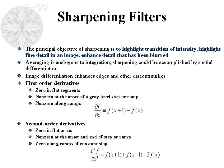
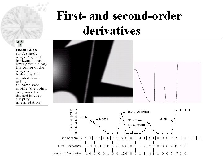
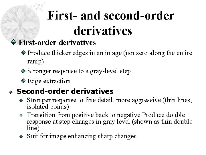
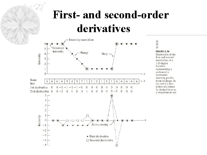
Sharpening Filters The principal objective of sharpening is to highlight transition of intensity, highlight fine detail in an image, enhance detail that has been blurred Averaging is analogous to integration, sharpening could be accomplished by spatial differentiation Image differentiation enhances edges and other discontinuities First-order derivatives Zero in flat segments Nonzero at the onset of a gray-level step or ramp Nonzero along ramps Second-order derivatives Zero in flat areas Nonzero at the onset and end of step or ramp Zero along ramps of constant slop

First- and second-order derivatives

First- and second-order derivatives First-order derivatives Produce thicker edges in an image (nonzero along the entire ramp) Stronger response to a gray-level step Edge extraction Second-order derivatives Stronger response to fine detail, more aggressive (thin lines, isolated points) Transition from positive back to negative Produce double response at step changes in gray level (shown as thin double line) Suit for image enhancing sharp changes

First- and second-order derivatives

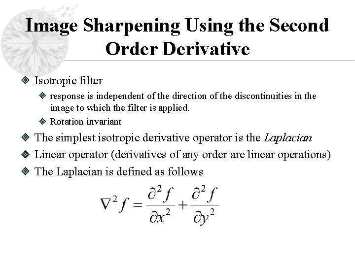
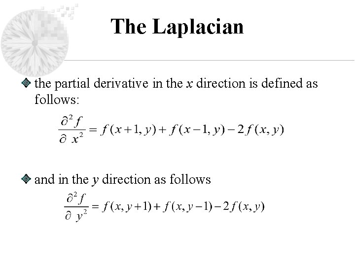
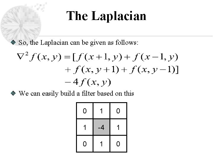
Image Sharpening Using the Second Order Derivative Isotropic filter response is independent of the direction of the discontinuities in the image to which the filter is applied. Rotation invariant The simplest isotropic derivative operator is the Laplacian Linear operator (derivatives of any order are linear operations) The Laplacian is defined as follows

The Laplacian the partial derivative in the x direction is defined as follows: and in the y direction as follows

The Laplacian So, the Laplacian can be given as follows: We can easily build a filter based on this 0 1 -4 1 0

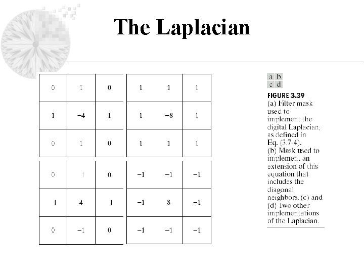
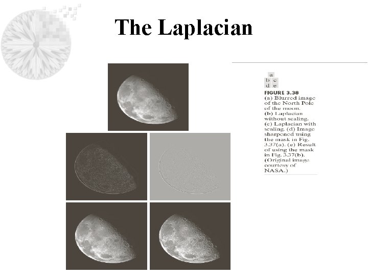
The Laplacian

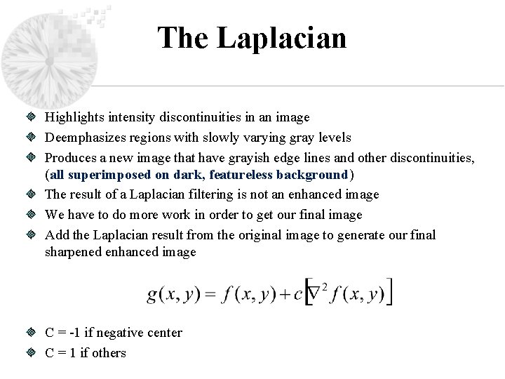
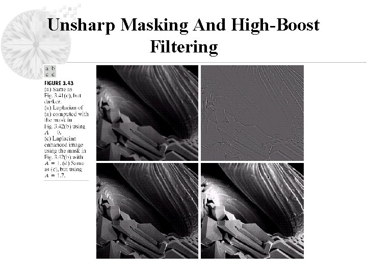
The Laplacian Highlights intensity discontinuities in an image Deemphasizes regions with slowly varying gray levels Produces a new image that have grayish edge lines and other discontinuities, (all superimposed on dark, featureless background) The result of a Laplacian filtering is not an enhanced image We have to do more work in order to get our final image Add the Laplacian result from the original image to generate our final sharpened enhanced image C = -1 if negative center C = 1 if others

The Laplacian

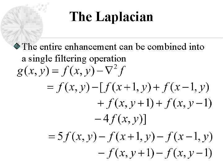
The Laplacian The entire enhancement can be combined into a single filtering operation

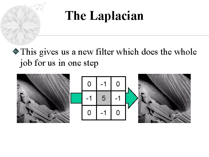
The Laplacian This gives us a new filter which does the whole job for us in one step 0 -1 5 -1 0

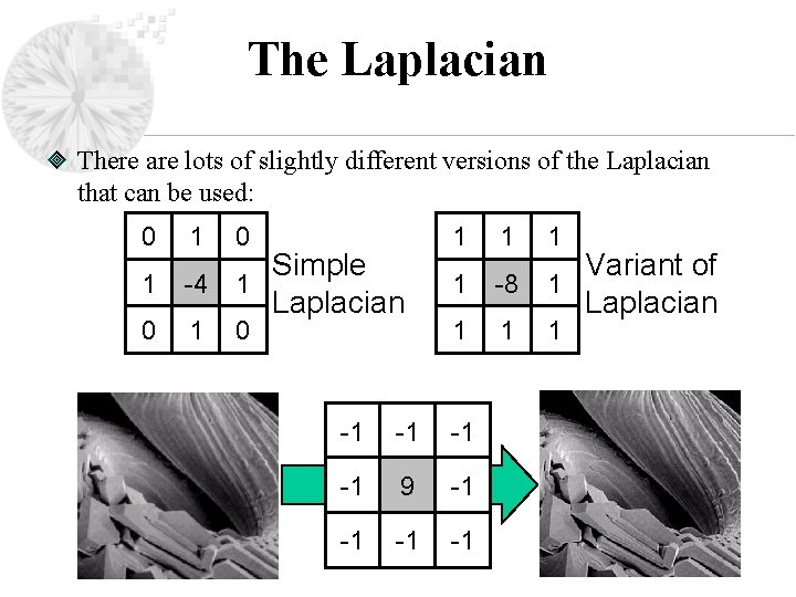
The Laplacian There are lots of slightly different versions of the Laplacian that can be used: 0 1 0 1 1 1 Simple 1 -4 1 Laplacian Variant of 1 -8 1 Laplacian -1 -1 9 -1 -1

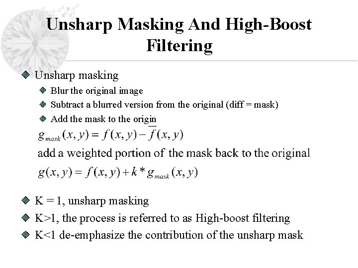
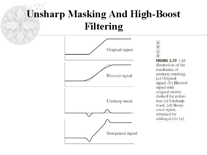
Unsharp Masking And High-Boost Filtering Unsharp masking Blur the original image Subtract a blurred version from the original (diff = mask) Add the mask to the origin K = 1, unsharp masking K>1, the process is referred to as High-boost filtering K<1 de-emphasize the contribution of the unsharp mask

Unsharp Masking And High-Boost Filtering

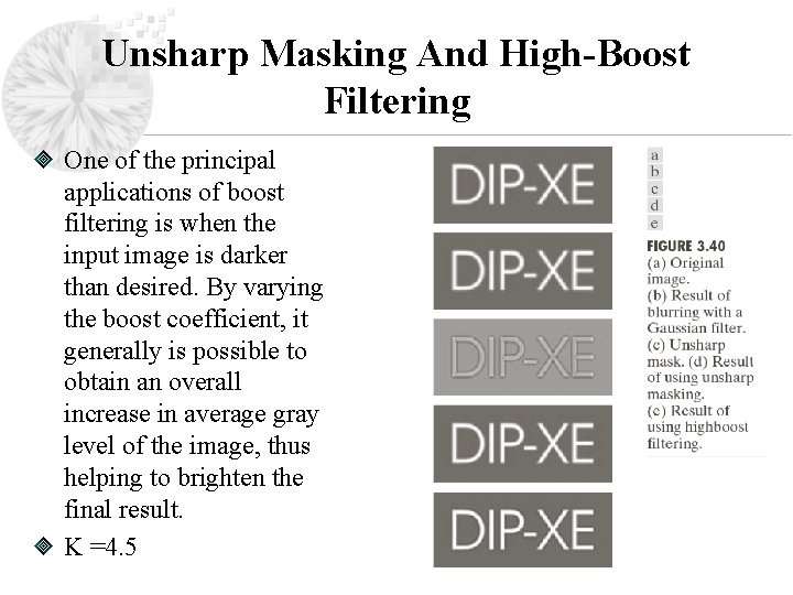
Unsharp Masking And High-Boost Filtering One of the principal applications of boost filtering is when the input image is darker than desired. By varying the boost coefficient, it generally is possible to obtain an overall increase in average gray level of the image, thus helping to brighten the final result. K =4. 5

Unsharp Masking And High-Boost Filtering

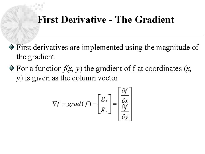
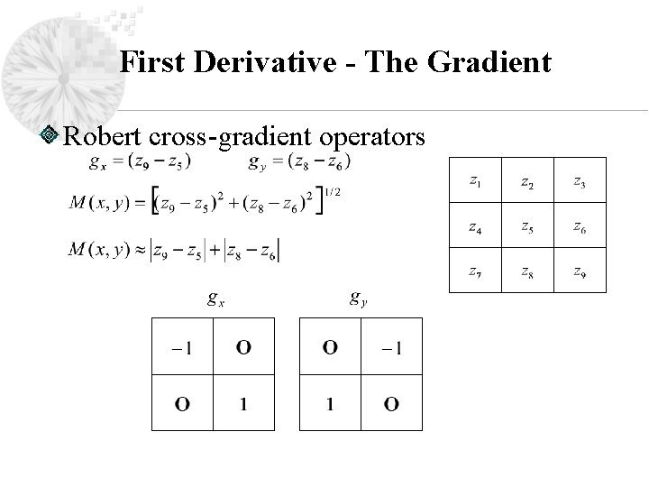
First Derivative - The Gradient First derivatives are implemented using the magnitude of the gradient For a function f(x, y) the gradient of f at coordinates (x, y) is given as the column vector

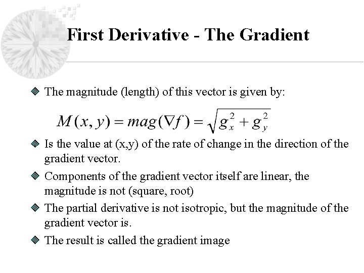
First Derivative - The Gradient The magnitude (length) of this vector is given by: Is the value at (x, y) of the rate of change in the direction of the gradient vector. Components of the gradient vector itself are linear, the magnitude is not (square, root) The partial derivative is not isotropic, but the magnitude of the gradient vector is. The result is called the gradient image

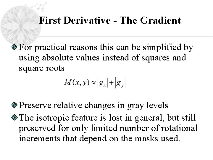
First Derivative - The Gradient For practical reasons this can be simplified by using absolute values instead of squares and square roots Preserve relative changes in gray levels The isotropic feature is lost in general, but still preserved for only limited number of rotational increments that depend on the masks used.

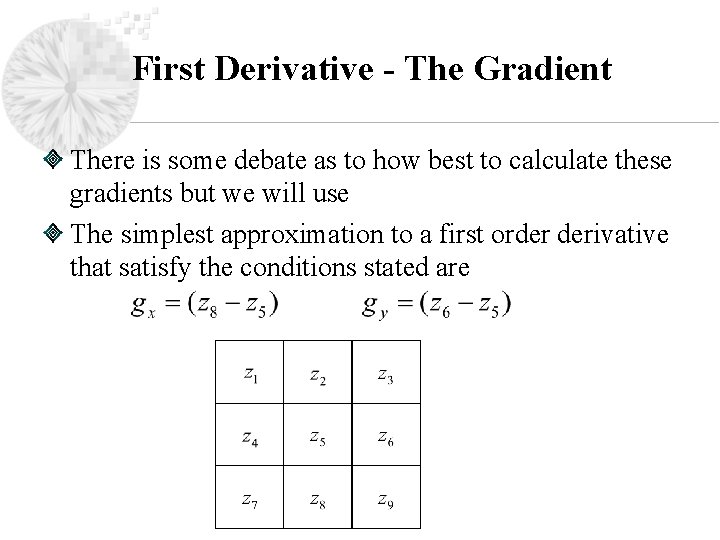
First Derivative - The Gradient There is some debate as to how best to calculate these gradients but we will use The simplest approximation to a first order derivative that satisfy the conditions stated are

First Derivative - The Gradient Robert cross-gradient operators

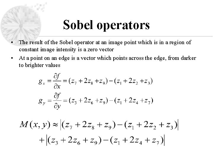
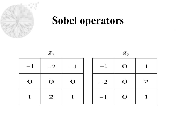
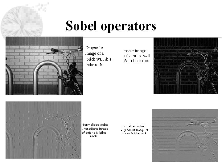
Sobel operators • The result of the Sobel operator at an image point which is in a region of constant image intensity is a zero vector • At a point on an edge is a vector which points across the edge, from darker to brighter values

Sobel operators

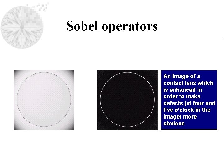
Sobel operators An image of a contact lens which is enhanced in order to make defects (at four and five o’clock in the image) more obvious

Sobel operators Grayscale image of a brick wall & a bike rack Normalized sobel y-gradient image of bricks & bike rack scale image of a brick wall & a bike rack Normalized sobel x-gradient image of bricks & bike rack

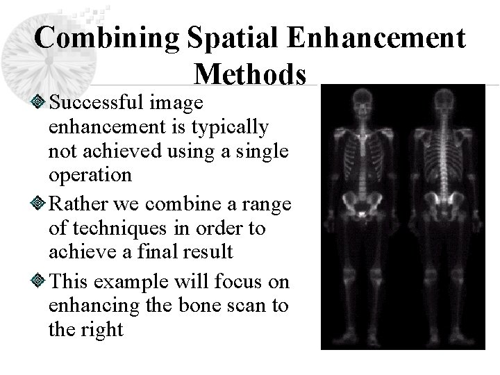
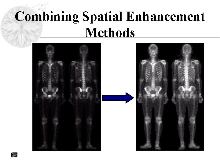
Combining Spatial Enhancement Methods Successful image enhancement is typically not achieved using a single operation Rather we combine a range of techniques in order to achieve a final result This example will focus on enhancing the bone scan to the right

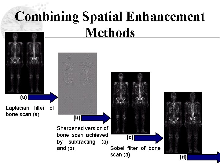
Combining Spatial Enhancement Methods (a) Laplacian filter of bone scan (a) (b) Sharpened version of bone scan achieved (c) by subtracting (a) Sobel filter of bone and (b) scan (a) (d)

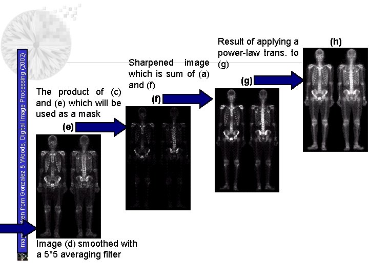
Images taken from Gonzalez & Woods, Digital Image Processing (2002) The product of (c) and (e) which will be used as a mask (e) Result of applying a power-law trans. to Sharpened image (g) which is sum of (a) (g) and (f) Image (d) smoothed with a 5*5 averaging filter (f) (h)

Combining Spatial Enhancement Methods