Image Processing Eri Prasetyo Wibowo Universitas Gunadarma Image

Image Processing Eri Prasetyo Wibowo Universitas Gunadarma
 1. a physical likeness or representation of a person, animal, or thing,")
Image (noun) 1. a physical likeness or representation of a person, animal, or thing, photographed, painted, sculptured, or otherwise made visible. 2. an optical counterpart or appearance of an object, as is produced by reflection from a mirror, refraction by a lens, or the passage of luminous rays through a small aperture and their reception on a surface. 3. a mental representation; idea; conception. 4. Psychology. a mental representation of something previously perceived, in the absence of the original stimulus. 5. form; appearance; semblance: We are all created in God's image. 6. counterpart; copy: That child is the image of his mother. 7. a symbol; emblem. . 14. Archaic. an illusion or apparition.

Digital Images • An image is a visual output of data stored in terms of a numeric, recordable elements. • Most digital images we use today are output in terms of a regular grid of pixels, referred to as a raster. • Intermediately the image can be stored in the form of lines, curves and filled areas, referred to as vector primitives. • All of these are eventually represented in a numerical way.

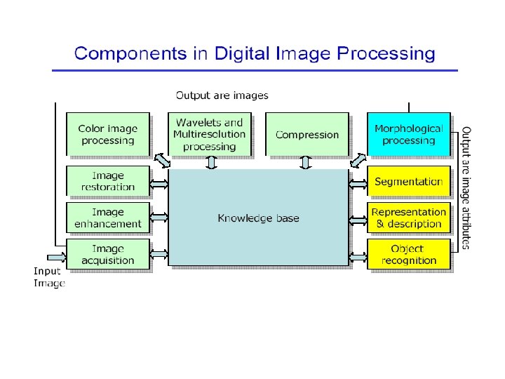
Related Areas Modelling Concepts Data / Models Rendering Image Processing Images Image Acquisition Computer Vision Real World
 •")
Image Processing • Some computer graphics operations involve manipulating 2 D images (bitmaps) • Image processing applies directly to the pixel grid and includes operations such as color correction, scaling, blurring, sharpening, etc. • Common example include digital photo processing and digital ‘painting’ programs (Adobe Photoshop…)

Image Processing CONCEPT MODEL Operations on Images IMAGE

Image Processing
 dari intensitas cahaya. Secara matematis disimbulkan")
Model Citra • Citra merupakan fungsi malar (kontinyu) dari intensitas cahaya. Secara matematis disimbulkan dengan f(x, y), dimana : – (x, y) : koordinat pada bidang dwi matra – F(x, y) : intensitas cahaya pada titik (x, y) • Nilai f(x, y) adalah hasil kali dari : – i(x, y) = jumlah cahaya yang berasal dari sumber, nilainya antara 0 sampai tak terhingga. – r(x, y) = derajat kemampuan objek memantulkan cahaya , nilainya antara 0 dan 1. – Jadi f(x, y) = i(x, y). r(x, y)

What is a Digital Image? • A digital image is a representation of a two -dimensional image as a finite set of digital values, called picture elements or pixels
 • Pixel values typically represent gray levels, colours,")
What is a Digital Image? (cont…) • Pixel values typically represent gray levels, colours, heights, etc • Remember digitization implies that a digital image is an approximation of a real scene 1 pixel
 • Common image formats include: – 1 sample")
What is a Digital Image? (cont…) • Common image formats include: – 1 sample per point (B&W or Grayscale) – 3 samples per point (Red, Green, and Blue) – 4 samples per point (Red, Green, Blue, and “Alpha”, a. k. a. Opacity) • For most of this course we will focus on grey-scale images

What is Digital Image Processing? • Digital image processing focuses on two major tasks – Improvement of pictorial information for human interpretation – Processing of image data for storage, transmission and representation for autonomous machine perception • Some argument about where image processing ends and fields such as image analysis and computer vision start

Digitalisasi Citra Supaya bisa diolah dengan komputer, citra harus direpsentasikan secara numerik dengan nilai diskrit. Citra digital dinyatakan dengan suatu matrik ukuran Nx. M. Masing-masing elemen disebut pixel (picture element) F(x, y) = f(0, 0) f(0, 1) …. f(0, m) f(1, 0) f(1, 1) …. f(1, M) : : f(N-1, 0) f(N-1, 1) : f(N-1, M-1) Indeks baris (i) dan indeks kolom (j) menyatakan koordinat titik pada citra, sedang f(i, j) merupakan intensitas (derajat keabuan) pada titik (i, j)

Perangkat keras sistem Visual Sensor Citra , untuk menangkap pantulan objek Jenisnya : CCD(charge coupled device) dan CMOS ( complementary metal-oxide semiconductor) ADC , mengkonversi sinyal analog menjadi sinyal digital Memori , untuk menyimpan data hasil konversi ADC dan memori dikemas dalam satu kesatuan yang disebut dengan penangkap bingkai citra ( image frame grabber)

Lingkup Pembahasan Image Enhancement Spatial Domain I. Point Processing a. b. c. d. e. f. g. h. Frequency Domain II. Mask Processing Image Negative Contrast Stretching Histogram Equalization - all grey level and all area - specific grey level (histogram specification) - local enhancement (specific part of the image) d. Image Subtracting e. Image Averaging
 g(x, y) Point Processing f(x, y) Area/Mask Processing g(x,")
Spatial Domain Methods f(x, y) g(x, y) Point Processing f(x, y) Area/Mask Processing g(x, y)

Point Processing Transformations • Convert a given pixel value to a new pixel value based on some predefined function.

I. Point Processing • Cara paling mudah untuk melakukan peningkatan mutu pada domain spasial adalah dengan melakukan pemrosesan yang hanya melibatkan satu piksel saja (tidak menggunakan jendela ketetanggaan) • Yang termasuk disini misalnya : • Citra negatif, • Contrast Stretching, • perataan histogram, • Image Substraction, • Image Averaging Ia. Citra Negatif Mengubah nilai grey-level piksel citra input dengan: Gbaru = 255 - Glama Hasilnya seperti klise foto
 = 255 -I(r, c)")
Negative Image • O(r, c) = 255 -I(r, c)

Citra asli Citra negatif Ib. Contrast Streching Mengubah kontras dari suatu image dengan cara mengubah greylevel piksel pada citra menurut fungsi s = T(r) tertentu r 1 ≤ r 2, s 1 ≤ s 2 r 1 = r 2, s 1 = s 2 tidak ada perubahan r 1 = r 2, s 1 = 0, s 2 = 255 tresholding menjadi citra biner dengan ambang r 1

Contrast Stretching or Compression • Stretch gray-level ranges where we desire more information (slope > 1). • Compress gray-level ranges that are of little interest (0 < slope < 1).

Thresholding • Special case of contrast compression

Intensity Level Slicing • Highlight specific ranges of gray-levels only. Same as double thresholding!

Bit-level Slicing • Highlighting the contribution made by a specific bit. • For pgm images, each pixel is represented by 8 bits. • Each bit-plane is a binary image

Logarithmic transformation • Enhance details in the darker regions of an image at the expense of detail in brighter regions.

Exponential transformation • Reverse effect of that obtained using logarithmic mapping.
 pada")
Ic. Histogram Equalization Histogram: diagram yang menunjukkan jumlah kemunculan grey level (0 -255) pada suatu citra Histogram processing: Gambar gelap: histogram cenderung ke sebelah kiri Gambar terang: histogram cenderung ke sebelah kanan Gambar low contrast: histogram mengumpul di suatu tempat Gambar high contrast: histogram merata di semua tempat Histogram processing: mengubah bentuk histogram agar pemetaan gray level pada citra juga berubah

Histogram Equalization • A fully automatic gray-level stretching technique. • Need to talk about image histograms first. . .

Image Histograms • An image histogram is a plot of the graylevel frequencies (i. e. , the number of pixels in the image that have that gray level).
 • Divide frequencies by total number of pixels to represent as")
Image Histograms (cont’d) • Divide frequencies by total number of pixels to represent as probabilities.
")
Image Histograms (cont’d)

Properties of Image Histograms • Histograms clustered at the low end correspond to dark images. • Histograms clustered at the high end correspond to bright images.
 • Histograms with small spread correspond to low contrast")
Properties of Image Histograms (cont’d) • Histograms with small spread correspond to low contrast images (i. e. , mostly dark, mostly bright, or mostly gray). • Histograms with wide spread correspond to high contrast images.
 Low contrast High contrast")
Properties of Image Histograms (cont’d) Low contrast High contrast

Histogram Equalization • The main idea is to redistribute the graylevel values uniformly.
 • In practice, the equalized histogram might not be completely flat.")
Histogram Equalization (cont’d) • In practice, the equalized histogram might not be completely flat.

Histogram Equalization in all grey level and all area Citra awal: 35554 54544 53444 45663 Citra Akhir: 19 9 95 95 9 55 91 5 55 5 9 10 10 1 n • Contoh : citra dengan derajat keabuan hanya berkisar 0 -10 n Derajat Keabuan 0 1 2 3 4 5 6 7 8 9 10 Kemunculan 0 0 0 3 8 7 2 0 0 Probabilitas Kemunculan 0 0. 15 0. 40 0. 35 0. 1 0 0 Sk 0 0. 15 0. 55 0. 90 1 1 1 SK * 10 0 1. 5 5. 5 9 10 10 10 Derajat keabuan baru 0 0 0 1 5 9 10 10 10
 • Jika pada point processing kita hanya melakukan operasi terhadap")
II. Mask Processing (1) • Jika pada point processing kita hanya melakukan operasi terhadap masing-masing piksel, maka pada mask processing kita melakukan operasi terhadap suatu jendela ketetanggaan pada citra. • Kemudian kita menerapkan (mengkonvolusikan) suatu mask terhadap jendela tersebut. Mask sering juga disebut filter. II. Mask Processing (2) 1 2 3 8 x 4 7 6 5 Contoh: Jendela ketetanggan 3 x 3, Nilai piksel pada posisi x dipengaruhi oleh nilai 8 tetangganya Perbedaan dengan point processing: pada point processing, nilai suatu piksel tidak dipengaruhi oleh nilai tetangga-tetangganya
 W 1 W 2 W 3 W 4 W 5")
II. Mask Processing (3) W 1 W 2 W 3 W 4 W 5 W 6 W 7 W 8 W 9 G 11 G 12 G 13 G 14 G 15 G 21 G 22 G 23 G 24 G 25 G 31 G 32 G 33 G 34 G 35 G 41 G 42 G 43 G 44 G 45 G 51 G 52 G 53 G 54 G 55 Contoh sebuah mask berukuran 3 x 3. Filter ini akan diterapkan / dikonvolusikan pada setiap jendela ketetanggaan 3 x 3 pada citra (anggap filter sudah dalam bentuk terbalik) G 22’ = w 1 G 11 + w 2 G 12 + w 3 G 13+ w 4 G 21 + w 5 G 22 + w 6 G 23 + w 7 G 31 + w 8 G 32 + w 9 G 33
 –")
Edge Detection • we discussed approaches for implementing – first-order derivative (Gradient operator) – second-order derivative (Laplacian operator) 42
 adalah perubahan nilai intensitas derajat keabuan yang cepat/tiba-tiba (besar)")
Definisi Tepi • Tepi (edge) adalah perubahan nilai intensitas derajat keabuan yang cepat/tiba-tiba (besar) dalam jarak yang singkat Profiles of image intensity edges § Step §Roof §Line

Tujuan Pendeteksian tepi • Untuk meningkatkan penampakan garis batas suatu daerah atau obyek di dalam citra. Teknik yang digunakan untuk pendeteksian tepi antara lain : §Operator gradien pertama ( differential gradient ) §Operator turunan kedua ( Laplacian )

Image gradient • The gradient of an image: • The gradient points in the direction of most rapid change in intensity The gradient direction is given by: • how does this relate to the direction of the edge? The edge strength is given by the gradient magnitude

Magnitude of gradient vector • Rumus 1: • Rumus 2: • Rumus 3: The discrete gradient • How can we differentiate a digital image f[x, y]? – Option 1: reconstruct a continuous image, then take gradient – Option 2: take discrete derivative (finite difference) 46

Gradient Masks 47
 Operator sobel")
• Digunakan operator sobel Tinjau pengaturan pixel disekitar pixel (x, y) Operator sobel adalah magnitude dari gradien yang dihitung dengan Atau M = |sx| + |sy| Turunan parsial dihitung dengan : Sx = (a 2+ca 3+a 4) – (a 0+ca 7+a 6) ; sy = (a 0+ca 1+a 2) – (a 6+ca 5+a 4) Dengan konstanta c=2 dalam bentuk mask, sx dan sy dinyatakan sebagai -1 0 1 Sx = -2 0 2 -1 0 1 1 Sy = 2 1 2 0 0 0 3 -1 -2 -1

• Contoh citra yang akan dilakukan pendeteksian tepi dengan operator sobel, -1 0 3 4 2 5 7 * * * 2 1 6 4 2 * 18 * Sx = -2 0 3 5 7 2 4 -1 0 4 2 5 7 1 2 5 1 6 9 citra awal citra hasil konvolusi 1 2 sx = 3 x(-1)+2 x(-2)+ 3 x(-1)+2 x(1)+6 x(2)+7 x(1) = 11 sy = 3 x(1)+4 x(2)+2 x(1)+3 x(-1)+5 x(-2)+7 x(-1) = -7 maka M = 18 Atau M = |sx| + |sy| • Operator lain adalah prewitt, dengan c = 1 -1 px= -1 -1 0 0 0 1 1 1 py = 1 0 -1 Sy = 2 0 0 1 2 1 1 0 3 -1 -2 -1

• Operator Robert disebut operator silang, gradien robert dalam arah x dan y dapat dihitung : R+(x, y) = f( x+1, y+1) – f(x, y) R-(x, y) = f(x, y+1) – f(x+1, y) f(x, y+1) f(x+1, y+1) f(x, y) f(x+1, y) Dalam bentuk mask operator adalah : 1 0 0 1 R+ = 0 -1 R- = -1 0 Nilai kekuatan tepi : G[f(x, y)] = |R+| + |R-| operator R+ adalah turunan berarah dalam arah 45 derajat, dan R- turunan berarah dalam arah 135 derajat

• Contoh deteksi tepi dengan robert : 4 2 4 4 2 5 1 3 2 4 7 3 2 5 8 5 4 6 7 6 1 5 9 1 3 citra awal f’[0, 0] = |4 -1| + |5 -2| = 6 6 4 3 0 2 8 1 2 7 4 5 5 6 2 8 3 6 7 5 6 1 5 9 1 3 citra hasil pendeteksian tepi

Diagonal edges with Prewitt and Sobel masks 52

The Laplacian • The Laplacian is defined as follows: • where the partial 1 st order derivative in the x direction is defined as follows: • and in the y direction as follows:
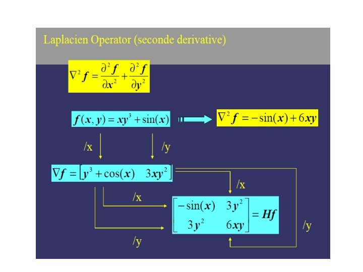
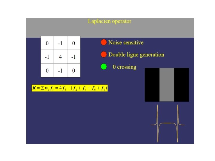
 • So, the Laplacian can be given as follows: • We")
The Laplacian (cont…) • So, the Laplacian can be given as follows: • We can easily build a filter based on this 0 1 -4 1 0
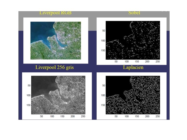
 • Applying the Laplacian to an image we get a new")
The Laplacian (cont…) • Applying the Laplacian to an image we get a new image that highlights edges and other discontinuities Original Image Laplacian Filtered Image Scaled for Display

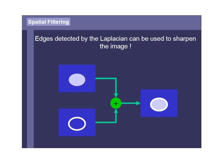
But That Is Not Very Enhanced! • The result of a Laplacian filtering is not an enhanced image • We have to do more work in order to get our final image • Subtract the Laplacian result from the original image to generate our final sharpened enhanced image Laplacian Filtered Image Scaled for Display

Laplacian Image Enhancement Original Image = Laplacian Filtered Image Sharpened Image • In the final sharpened image edges and fine detail are much more obvious

Simplified Image Enhancement • The entire enhancement can be combined into a single filtering operation
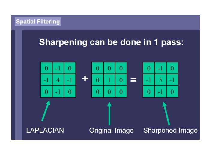
 • This gives us a new filter which does the")
Simplified Image Enhancement (cont…) • This gives us a new filter which does the whole job for us in one step 0 1 5 1 0

Variants on the Simple Laplacian • There are lots of slightly different versions of the Laplacian that can be used: 0 1 -4 1 0 Simple Laplacian 1 1 -8 1 1 1 1 9 1 1 Variant of Laplacian
- Slides: 65