Hypothesis testing Dr David Field Summary Null hypothesis

Hypothesis testing Dr David Field

Summary • • Null hypothesis and alternative hypothesis Statistical significance (p-value, alpha level) One tailed and two tailed predictions What is a true experiment? – random allocation to conditions • Outcomes of experiments – Type I and Type II error • Interpreting 95% confidence intervals – are two samples from the same population?

Comparing two samples • Lectures 1 and 2, and workshop 1 focused on describing a single variable, which was a sample from a single population • Today’s lecture will consider what happens when you have two variables (samples) • The researcher usually wants to ask if the two samples are from the same population or two different populations? • We’ll also consider examples where there is a single sample, but two variables have been measured to assess the relationship between them

Maths exam performance

Maths exam performance

Maths exam performance

Interpreting confidence intervals on graphs • If the 95% confidence intervals for two means do not overlap then we treat the difference between the means as real (reliable / significant / the null hypothesis can be rejected) – These terms will be explained shortly • If the 95% confidence intervals around two means do overlap, there might be a real difference, but the graph does not itself establish this – To decide, an inferential statistical test is required (t test lecture) • Warning: some journal articles plot 1 SE rather than 95% confidence on graphs – Watch out for this as 1 SE is effectively a 68% confidence interval rather than a 95% confidence interval – In this case the rule at the top of this slide does not apply

Hypothesis and null hypothesis • Imagine some researchers have a theory that eating fruit and vegetables improves brain function • They hypothesize that people who eat more fruit and vegetables will perform better in exams • The null hypothesis is that there will be no relationship at all between fruit and vegetable consumption and exam performance – The null hypothesis is required in order to set up statistical tests that can find support for the hypothesis – The null hypothesis is very exact, it means exactly no relationship – This exact property allow the null hypothesis to be used to set up an imaginary “null distribution” for statistical purposes • The hypothesis itself is often referred to as the “alternative hypothesis” because if you can show that the null hypothesis is false then this is evidence for the alternative

• Imagine the researchers test their hypothesis by sampling 12 students • This graph is a scatterplot • In the sample, exam performance increases as fruit & vegetable consumption increases. Scatterplot:

• Visually, the evidence in the previous slide is strong, but it is based upon a small sample of 12 individuals • We need a way of quantifying our confidence that are that the pattern in the sample is a true reflection of the pattern in the population

random sample null population distribution population?

Null hypothesis testing • In an ideal world, we’d directly estimate the probability that the population conforms to the alternative hypothesis given the sample – “We are 95% certain that there is a positive relationship between eating fruit and vegetables and exam performance” • This is not possible using classical statistics • Which is because there an infinite number of possible alternative hypothesis population distributions • But there is only 1 null population distribution, which makes it possible to calculate the probability that the data could be a random sample from it

Null hypothesis testing • If the probability that the data could be a random sample from the null distribution is less than 5% (1 in 20) you can reject the null hypothesis as false – this indirectly supports the alternative hypothesis, which is never directly tested • If the probability that the data could be a random sample from the null distribution is greater than 5% (1 in 20) you fail to reject the null hypothesis – failing to reject the null hypothesis is not the same as saying that the null hypothesis is true – statistics never allow you to say that the null hypothesis is true

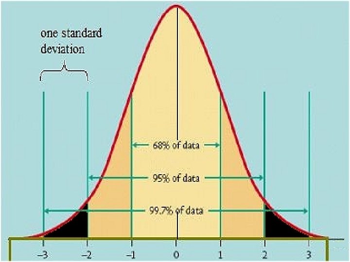
Why 0. 05 (5%, or 1 in 20)? • This is somewhat arbitrary – 0. 05 is called the alpha level – sometimes 0. 01 is used instead • 0. 05 does produce a good balance between the probability of a researcher making Type I error the probability of making a Type II error – see later for meaning of these types of error • What you need to understand about probability values (p values) is that – – p = 100% = certainty p = 0. 1 = 10% = 1 in 10 p = 0. 05 = 5% = 1 in 20 p = 0. 01 = 1% = 1 in 100

sample N = 12 null population distribution • How can we quantify the probability of obtaining a sample like the one we have from the null distribution? – Using sampling distributions – Imagine drawing a very large number of samples, each with N = 12 from the null distribution – A few of them would look very similar to the actual sample from the real population – Perhaps 1% of the samples would look like the top left graph. – Therefore, the p value of the data would be 1%

sample N = 12 null population distribution • But what does similar mean? – Very few random samples from the null distribution would be exactly the same as the sample obtained from the real population – In this example, what defines the null distribution is that there is no relationship at all between exam performance and fruit consumption – A statistic called a correlation coefficent quantifying the strength of the relationship between two variables can be calculated – It has a value of 0 for the null distribution

sample N = 12 • But what does similar mean? null population distribution – For each sample the correlation statistic can be calculated – Two samples can both have a correlation of 0. 5 between exam performance and fruit consumption without being identical to each other – Therefore, the null distribution is defined in terms of values of statistics (like the correlation coeffient) – If the obtained sample has a correlation of 0. 5 you can calculate the p of a single sample from the null distribution having a correlation of 0. 5 or higher – If p < 0. 05 you would reject the null hypothesis – Details of statistics that can be converted to p values are covered in later lectures

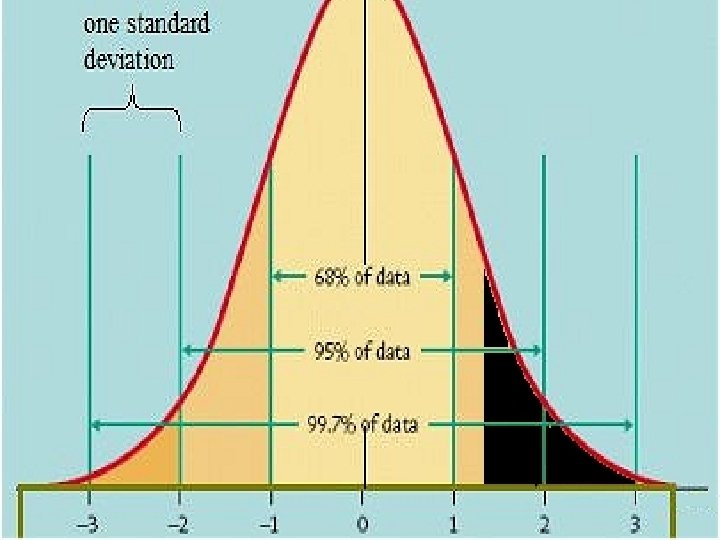
One tailed and two tailed hypotheses • In the example the researchers predicted that exam performance would improve as fruit and vegetable consumption increases – This is a one directional hypothesis (one tailed) – Another group of researchers, funded by a junk food manufacturer, might predict the opposite • It is also possible to predict that one variable will influence another, without specifying a direction – e. g. , people who eat a lot of fruit and vegetables will perform differently in exams than people who eat a small amount of fruit and vegetables – This is a two tailed hypothesis

One tailed and two tailed hypotheses • Where do the names “one tailed” and “two tailed” come from?

One tailed and two tailed hypotheses • This slide and the next one should be referred to when writing lab reports • SPSS, the program you will use for statistical analysis always reports two tailed significance levels • If you have a one tailed hypothesis you can divide the significance value SPSS gives you in half – p = 0. 08 becomes p = 0. 04 – It is important to do this, as many results with small samples will be significant on a one tailed test but not a two tailed test – 0. 08 > 0. 05 (fail to reject null), 0. 04 < 0. 05 (reject null) • But, do not divide the value of the statistic (e. g. , “t” or “r”) SPSS reports in half

Reporting statistical significance 1) Is the p-value > 0. 05? • Remember to divide by 2 first if one tailed 2) If the answer to 1) above is “yes” then you can write “t(29) = 1. 2, NS” • • you will learn where the 29 and the 1. 2 come from in the t test lecture NS stands for “non significant” 3) If the answer to 1) above is “no” then you can write something like “t(29) = 4. 3, p = 0. 03” • • • the value of p written here is the same number you tested in 1) above In this case you are reporting a statistically significant result This way of reporting is called “reporting exact p values”

Meaning of “statistical significance” • “Significant” does not mean “important” • Significance is just the probability of obtaining a result as extreme or more extreme than the sample data you have assuming the underlying population conforms to the null distribution, in which the mean is zero • Recall from lecture 2 and workshop 1 that the SE and 95% confidence interval around a sample mean reduces as sample size increases – Large samples will have very small SE making it is very easy to achieve p of null hypothesis < 0. 05 – With a large sample, if the null hypothesis were true, then producing a result even slightly different from the null hypothesis by random sampling is very unlikely • For example, if you sample maths scores for 1000 boys and 1000 girls – null hypothesis is that boys and girls score the same – If you get a mean of 68% for girls and 67% for boys, this small difference can easily reach statistical significance with N = 2000 – But such a difference is not important

Experiments • In the fruit and vegetables example the researchers randomly sampled some students and measured two variables – the relationship was plotted – Next term you will learn how to calculate “correlations” to statistically describe this kind of data • In the boys and girls maths performance example the researchers compared a random sample of boys with a random sample of girls – they were looking for a difference between groups • Neither of these research designs constitute a true experiment

Experiments • In the fruit and vegetables example exam performance increased as a function of fruit and vegetable intake – but the researchers did not manipulate the amount of fruit and vegetables eaten by participants – perhaps fruit and vegetable intake increases as exercise increases – and perhaps exam performance also increases as exercise increases – exercise is a third variable that might potentially cause the changes in the other two • You can’t infer causality by observing a relationship (correlation) between two variables

Experiments • The boys versus girls case seems more clear cut, but in reality this is still a correlational design – The researchers were not able to decide if each participant would be male or female, they just come that way – This opens up the possibility that the male / female dichotomy might be correlated with a third variable that is the true explanation of the difference in maths between boys and girls – For example, perhaps shorter people are better at maths, and girls are shorter than boys on average – Height is a confounding variable because it can potentially provide an alternative explanation of the data that competes with the researchers hypothesis – This is an implausible example, but it makes the point that the researcher is not really in control of the experiment when comparing groups that are predefined such as boys vs girls, old vs young,

Experiments • In a true experiment, the researchers can manipulate the variables, e. g. they decide how much fruit and vegetables each participant eats • Things that researchers can manipulate are called independent variables (IV) • The thing that is measured because it is hypothesized that the independent variable has a causal influence on it is called the dependent variable (DV) • In a true experiment participants are almost always randomly allocated to conditions.

Random allocation • Researchers think that supplementing diet with 200 g of blueberries per day will improve exam performance compared to equivalent calories consumed as sugar cubes • But exam performance will also be influenced by other factors, such as IQ, and number of hours spent studying • If each participant in the total sample is randomly allocated to blueberries or sugar cubes, then with enough participants the mean IQ in the two samples and the mean number of hours studied will turn out to be about equal – because these two variables are “equalised” across the two levels of the IV by randomization they will not contribute to any difference in mean exam scores between the sugar cube and blueberry groups – Random allocation to conditions even protects the researcher against the influence of confounds he/she has not thought of! • If the blueberry group have higher exam scores than the sugar cube group the difference must be caused by the IV

Random allocation • IQ and number of hours studied will not influence the mean exam score in the blueberry group or the sugar cube group • We will be able to plot two frequency histograms of the exam scores, one for each group – and calculate the SD • Can IQ scores and hours spent studying influence the SD of the scores in the two groups? – imagine we run the experiment once using a sample containing great variation in IQ and study hours – imagine we run the experiment again using a sample selected so that the IQ’s only vary between 100 and 110, and everyone has similar studying habits • What implication could this have for the ability of the experiment to produce a statistically significant result?

Blueberries mean 57. 3 SD 10. 6 % N = 29 Sugar cubes 51. 4 % SD 12. 3 % N = 29

The null hypothesis in a true experiment • Begin with a single sample from a single population • Randomly divide the sample between the two levels of the IV • You now have two samples • The hypothesis is that the IV is successful in causing the two samples to come from two statistically separate populations (e. g. of exam scores) • The null hypothesis is that the two samples remain as samples from a single population (e. g. of exam scores)

Outcomes of Experiments reality in population null is false experiment outcome reject null p < 0. 05 fail to reject null p > 0. 05 NS null is “true”

Outcomes of Experiments reality in population null is false experiment outcome reject null fail to reject null is “true” true positive true negative

Outcomes of Experiments reality in population experiment outcome reject null fail to reject null is false null is “true” true positive false positive (Type I error) true negative

Outcomes of Experiments reality in population experiment outcome reject null fail to reject null is false null is “true” true positive P value of experiment IS the probability of a Type I error true negative

Outcomes of Experiments reality in population experiment outcome null is false null is “true” reject null true positive P value of statistic is probability of a Type I error fail to reject null false negative (Type II error) true negative

Outcomes of Experiments reality in population experiment outcome null is false null is “true” reject null true positive P value of statistic is probability of a Type I error fail to reject null Probability of Type II true error cannot negative be assessed

Relationship between Type I and Type II error • Conventionally, we use 0. 05 as a threshold (or cut off, or criterion) to decide whether we reject the null hypothesis or not • A researcher can use a more conservative, stricter, threshold, such as 0. 01 (1%) – this reduces the chance of a researcher publishing a Type I error – but it increases the chance of a Type II error • The only way to find out if an experimental result is a Type 1 error is to replicate (repeat) it – p of two consecutive type I errors is 0. 05 * 0. 05 = 0. 0025 • One reason that the 0. 05 alpha level is conventionally adopted is because it produces a good compromise between the probability of a Type I error and the probability of a Type II error occurring