Null Hypothesis and Alternate Hypothesis A person has

帰無仮説と対立仮説 Null Hypothesis and Alternate Hypothesis • A person has headache （pain in head) Before it, he drank a glass of bad wine. • Alternate Hypothesis: what is susceptive; The wine was the cause of the pain. (guilty) • Null Hypothesis: Opposite to that hypothesis; The wine was not the cause of the pain. (innocent) 2

棄却と採択 Rejection of the Null Hypothesis • When we permit the Null Hypothesis, the probability of the realized event is calculated. – Calculate the probability of headache when he did not drink such a wine. • If the probability is too small (smaller than your critical probability), you can reject the nullhypothesis and approve the alternate hypothesis. – The wine was the cause of the pain. (guilty) • If the probability is not too small, you cannot say anything. (not actively approve the null hypothesis). – The wine was not the cause of the pain. (innocent) 3

連続変数と棄却域 Critical Value for Continuous Variable • If he had headache with certain large probability, when drinking no wine, we cannot reject the Null Hypothesis. • We take a continuous variable such as headache duration, we can set the critical region, more easily, based on the usual probability density. Probability Density under the Null Hypothesis 0. 05 No-ache Ache 60 min Duration of headache 4

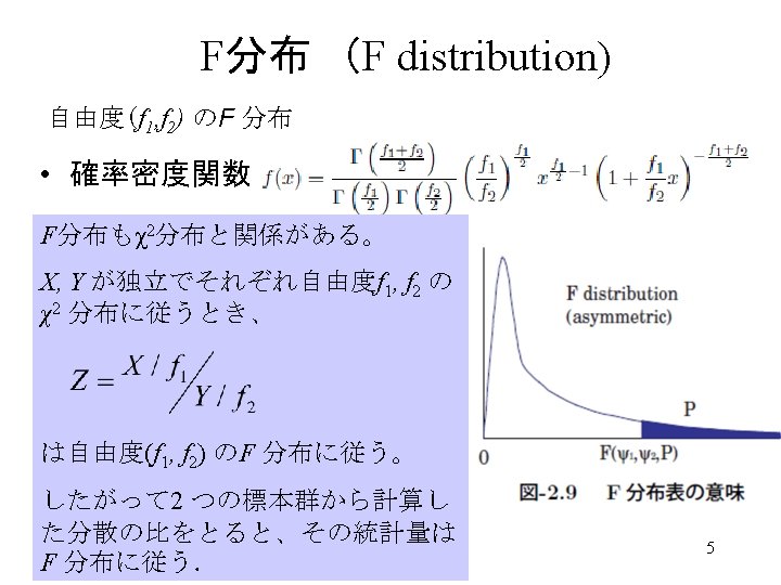
　F分布表　（F distribution) 6

回帰による記述（説明）力の検定 ANOVA Test of overall fitness 回帰平方和が誤差平方和に比べ、大きな意味を持っているか？ Does RSS have remarkable meaning comparing to ESS? 帰無仮説：回帰平方和は誤差平方和と同程度の大きさ （回帰式は、誤差に比べて大きな説明力はない） Null Hypothesis: RSS have similar meaning with ESS. (Ratio of Two Variances originated from same population obeys to F-distribution) 対立仮説：回帰平方和は誤差平方和より大きい 　（回帰式によって誤差よりもかなり大きい部分が説明できた） Alternative Hypothesis. : RSS have larger meaning than ESS. 9

回帰による記述（説明）力の検定例 帰無仮説：回帰平方和は誤差平方和と同程度の大きさ （回帰式は、誤差に比べて大きな説明力はない） Rejected (棄却） Null Hypothesis: RSS have similar meaning with ESS. (Ratio of Two Variances originated from same population obeys to F-distribution) 対立仮説：回帰平方和は誤差平方和より大きい採択Approved 　（回帰式によって誤差よりもかなり大きい部分が説明できた） Alternative Hypothesis. : RSS have larger meaning than ESS. Multiple R-squared: 0. 9511, Adjusted R-squared: 0. 9348 10 F-statistic: 58. 37 on 2 and 6 DF, p-value: 0. 0001168

7. 1一元配置法(対応なし)ｐ. 159 Single Factor Model • Are grade points different between groups? • A B C D 15 9 18 14 18 13 8 8 12 7 10 6 11 7 12 10 7 3 5 7 11

変動の分解Decomposition of Variance A B C D 15 13 10 10 9 8 6 7 18 8 11 3 14 12 7 5 18 7 12 7 10 10 10 10 10 +5 -1 +8 +4 +8 +3 -2 -2 +2 -3 0 -4 +1 -3 +2 0 -3 -7 -5 -3 ＝ ＋ 観測値Observation 全体平均Total Mean A B C D +5 +3 0 -1 -2 -4 +8 -2 +1 +4 +2 -3 +8 -3 +2 0 -3 -7 -5 -3 4. 8 4. 8 -0. 4 -0. 8 -3. 6 ＝ 全体変動Total Error 全体変動 Total error A ＋ B C D 0. 2 3. 4 0. 8 3. 6 -5. 8 -1. 6 -3. 2 0. 6 3. 2 -1. 6 1. 8 -3. 4 -0. 8 2. 4 -2. 2 -1. 4 3. 2 -2. 6 2. 8 -0. 6 12 群間平均 inter-group 群内変動Inner Error

平方和の評価 Sum of Squares and Variance A B C D +5 +3 0 -1 -2 -4 +8 -2 +1 +4 +2 -3 +8 -3 +2 0 -3 -7 -5 -3 4. 8 4. 8 -0. 4 -0. 8 -3. 6 ＝ A ＋ 全体変動Total Error 群間平均Inter-group Sum of Sq. 平方和　322 平方和　184 Var. 分散 16. 94＝ 322/19 分散 61. 3 -184/3 D. F. 自由度 19＝ 20 -1 B C D 0. 2 3. 4 0. 8 3. 6 -5. 8 -1. 6 -3. 2 0. 6 3. 2 -1. 6 1. 8 -3. 4 -0. 8 2. 4 -2. 2 -1. 4 3. 2 -2. 6 2. 8 -0. 6 群内変動Inner-error 平方和　138 分散 8. 6=138/16 自由度 3＝ 4 -1 自由度 16=4(5 -1) 13 F=61. 33/8. 625=7. 11

　F分布表　（F distribution) 3. 24 7. 111＞F(0. 05: 3, 16)＝ 3. 24 7. 11 Under the null-hypothesis, The Ratio of Variance goes beyond the observed value (7. 111) with Probability smaller than 0. 05. You can reject the null-hypothesis: 14 The inter-group variation is statistically different from the inner-group.

Rによる計算　aov() Testgrade <-c(15, 9, 18, 14, 18, 13, 8, 8, 12, 7, 10, 6, 11, 7, 12, 10, 7, 3, 5, 7) Methods <-c(rep('A', 5), rep('B', 5), rep('C', 5), rep('D', 5)) oneway. test(Testgrade~Methods, var. equal=TRUE) One-way analysis of means data: Testgrade and Methods F = 7. 1111, num df = 3, denom df = 16, p-value = 0. 002988 summary(aov(Testgrade~Methods)) Df Sum Sq Mean Sq F value Pr(>F) Methods 3 184 61. 33 7. 111 0. 00299 ** Residuals 16 138 8. 63 --Signif. codes: 0 ‘***’ 0. 001 ‘**’ 0. 01 ‘*’ 0. 05 ‘. ’ 0. 1 ‘ ’ 1

7. 2一元配置法(対応あり)ｐ. 175 Single factor Model • 3科目に対する好意度の評価 • How Favorite are they feel for three subjects Student Algebra Calculus Statistics Akita Inoue Uchida Egawa Otani 7 8 9 5 6 5 4 7 1 3 8 6 7 2 5 16

変動の分解Decomposition A I U E O A C S 7 8 9 5 6 5 4 7 1 3 8 6 7 2 5 観測値Observed 全体 ＝ 変動 Total Error A I U E O A I ＝U E O A C S 5. 53 5. 53 ＋ A I U E O C S 1. 46 -1. 53 0. 06 1. 46 -1. 53 1. 46 -1. 53 0. 06 条件(科目間) A A 1. 13 I 0. 46 ＋ U 2. 13 E -2. 86 O -0. 86 C S 1. 46 -0. 53 2. 46 -1. 53 0. 46 3. 46 1. 46 -0. 53 -4. 53 -3. 53 0. 46 -2. 53 -0. 53 全体変動 Total error 全体平均Total Mean A A C S 1. 13 0. 46 2. 13 -2. 86 -0. 86 A A -1. 13 I 0. 53 ＋ U -0. 13 E 0. 86 O -0. 13 個人差(個人間) C S -0. 13 1. 26 -0. 46 -0. 06 0. 86 -0. 73 -0. 13 -0. 26 17 Error(残差)

平方和の評価 Evaluation with Variances 全体変動 ＝ Total Error A I U E O A C S 1. 46 -1. 53 0. 06 1. 46 -1. 53 1. 46 -1. 53 0. 06 A A 1. 13 I 0. 46 ＋ U 2. 13 E -2. 86 O -0. 86 Inter-column Sum of Sq. 平方和　73. 73 D. F. 自由度 14＝ 15 -1 平方和　22. 53 C S 1. 13 0. 46 2. 13 -2. 86 -0. 86 Inter-row 平方和　45. 06 A A -1. 13 I 0. 53 ＋ U -0. 13 E 0. 86 O -0. 13 C S -0. 13 1. 26 -0. 46 -0. 06 0. 86 -0. 73 -0. 13 -0. 26 Error(残差) 平方和　6. 133 分散 11. 267 分散　0. 767 自由度 2＝ 3 -1 自由度 4＝ 5 -1 自由度 8=4(3 -1) Fo=11. 267/0. 767=14. 69>F(2, 8, 0. 05)=4. 64 Fo=11. 267/0. 767=14. 69>F(4, 8, 0. 05)=3. 84 18

Rによる計算　aov() Preferences <-c(7, 8, 9, 5, 6, 5, 4, 7, 1, 3, 8, 6, 7, 2, 5) Subjects <-c(rep('AL', 5), rep('CL', 5), rep('ST', 5)) Person <-rep(c('AK', 'IN', 'UC', 'EG', 'OT'), 3) summary(aov (Preferences~Subjects)) Df Subjects 2 Residuals 12 Sum Sq Mean Sq 22. 53 11. 267 51. 20 4. 267 F value Pr(>F) 2. 641 0. 112

Rによる計算　aov() summary(aov(Preferences~Person)) Df Sum Sq Mean Sq F value Pr(>F) Person 4 45. 067 11. 267 3. 9302 0. 03603 * Residuals 10 28. 667 2. 867 --Signif. codes: 0 ‘***’ 0. 001 ‘**’ 0. 01 ‘*’ 0. 05 ‘. ’ 0. 1 ‘ ’ 1 summary(aov(Preferences~Subjects+Person) ) Df Sum Sq Mean Sq F value Pr(>F) Subjects 2 22. 533 11. 267 14. 696 0. 002095 ** Person 4 45. 067 11. 267 14. 696 0. 000931 *** Residuals 8 6. 133 0. 767 --Signif. codes: 0 ‘***’ 0. 001 ‘**’ 0. 01 ‘*’ 0. 05 ‘. ’ 0. 1 ‘ ’ 1