SUMMARY Hypothesis testing Selfengagement assesment Null hypothesis song

SUMMARY Hypothesis testing

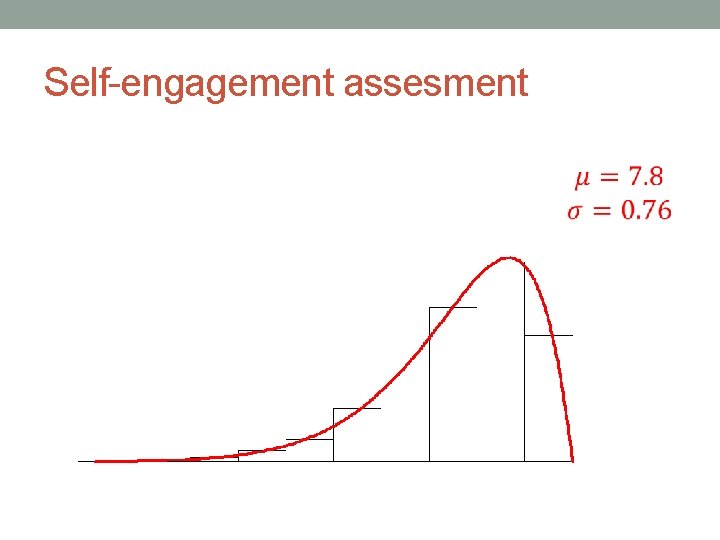
Self-engagement assesment

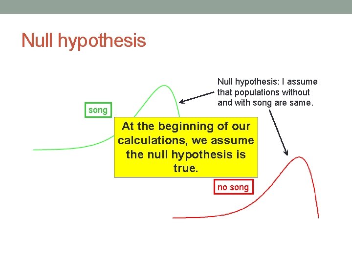
Null hypothesis song Null hypothesis: I assume that populations without and with song are same. At the beginning of our calculations, we assume the null hypothesis is true. no song

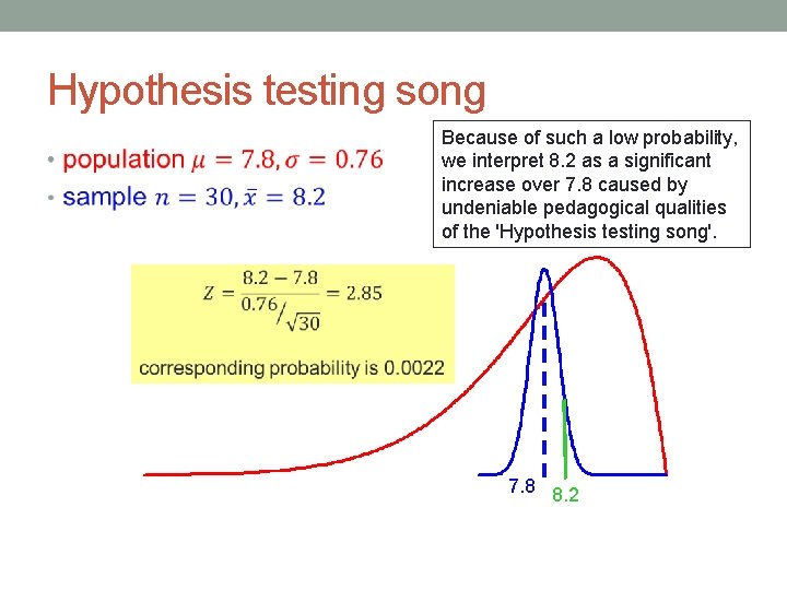
Hypothesis testing song • Because of such a low probability, we interpret 8. 2 as a significant increase over 7. 8 caused by undeniable pedagogical qualities of the 'Hypothesis testing song'. 7. 8 8. 2

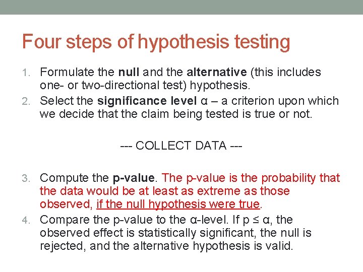
Four steps of hypothesis testing 1. Formulate the null and the alternative (this includes one- or two-directional test) hypothesis. 2. Select the significance level α – a criterion upon which we decide that the claim being tested is true or not. --- COLLECT DATA --3. Compute the p-value. The p-value is the probability that the data would be at least as extreme as those observed, if the null hypothesis were true. 4. Compare the p-value to the α-level. If p ≤ α, the observed effect is statistically significant, the null is rejected, and the alternative hypothesis is valid.

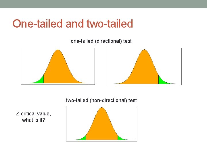
One-tailed and two-tailed one-tailed (directional) test two-tailed (non-directional) test Z-critical value, what is it?

NEW STUFF

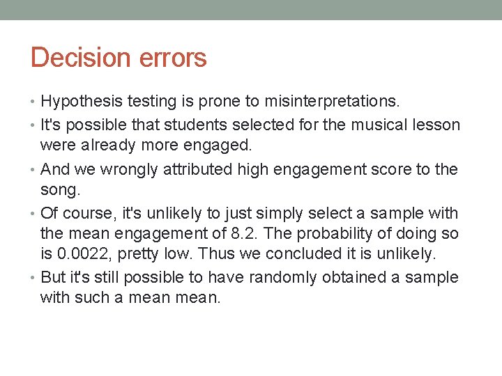
Decision errors • Hypothesis testing is prone to misinterpretations. • It's possible that students selected for the musical lesson were already more engaged. • And we wrongly attributed high engagement score to the song. • Of course, it's unlikely to just simply select a sample with the mean engagement of 8. 2. The probability of doing so is 0. 0022, pretty low. Thus we concluded it is unlikely. • But it's still possible to have randomly obtained a sample with such a mean.

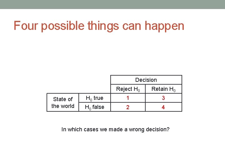
Four possible things can happen Decision State of the world Reject H 0 Retain H 0 true 1 3 H 0 false 2 4 In which cases we made a wrong decision?

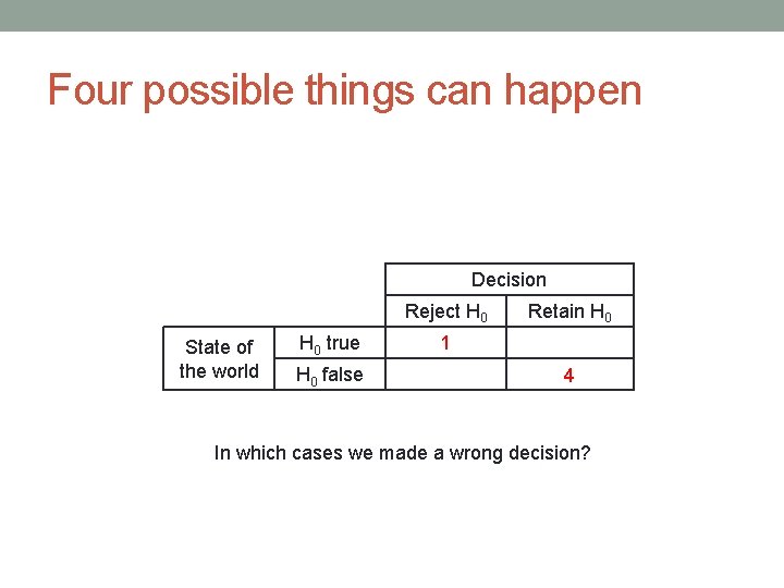
Four possible things can happen Decision Reject H 0 State of the world H 0 true H 0 false Retain H 0 1 4 In which cases we made a wrong decision?

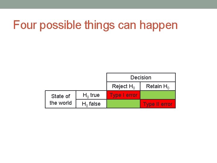
Four possible things can happen Decision Reject H 0 State of the world H 0 true H 0 false Retain H 0 Type I error Type II error

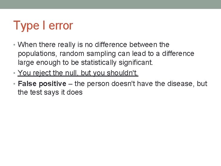
Type I error • When there really is no difference between the populations, random sampling can lead to a difference large enough to be statistically significant. • You reject the null, but you shouldn't. • False positive – the person doesn't have the disease, but the test says it does

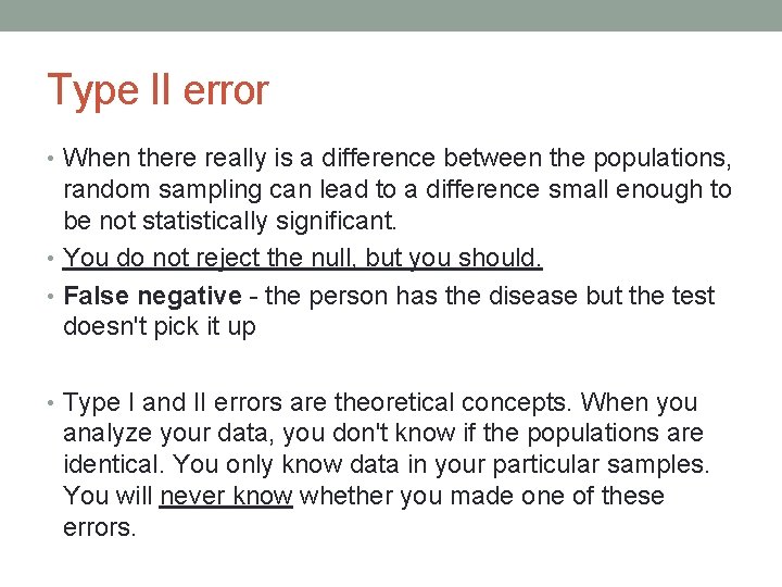
Type II error • When there really is a difference between the populations, random sampling can lead to a difference small enough to be not statistically significant. • You do not reject the null, but you should. • False negative - the person has the disease but the test doesn't pick it up • Type I and II errors are theoretical concepts. When you analyze your data, you don't know if the populations are identical. You only know data in your particular samples. You will never know whether you made one of these errors.

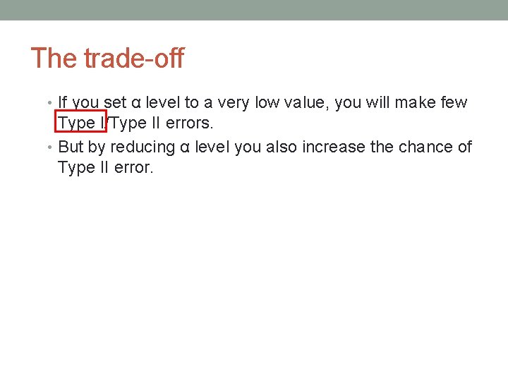
The trade-off • If you set α level to a very low value, you will make few Type I/Type II errors. • But by reducing α level you also increase the chance of Type II error.

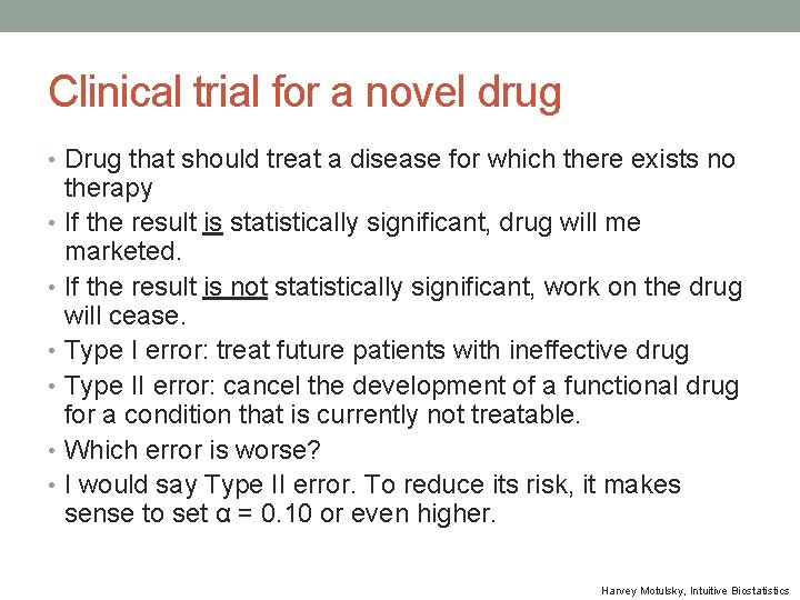
Clinical trial for a novel drug • Drug that should treat a disease for which there exists no therapy • If the result is statistically significant, drug will me marketed. • If the result is not statistically significant, work on the drug will cease. • Type I error: treat future patients with ineffective drug • Type II error: cancel the development of a functional drug for a condition that is currently not treatable. • Which error is worse? • I would say Type II error. To reduce its risk, it makes sense to set α = 0. 10 or even higher. Harvey Motulsky, Intuitive Biostatistics

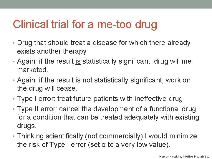
Clinical trial for a me-too drug • Drug that should treat a disease for which there already exists anotherapy • Again, if the result is statistically significant, drug will me marketed. • Again, if the result is not statistically significant, work on the drug will cease. • Type I error: treat future patients with ineffective drug • Type II error: cancel the development of a functional drug for a condition that can be treated adequately with existing drugs. • Thinking scientifically (not commercially) I would minimize the risk of Type I error (set α to a very low value). Harvey Motulsky, Intuitive Biostatistics

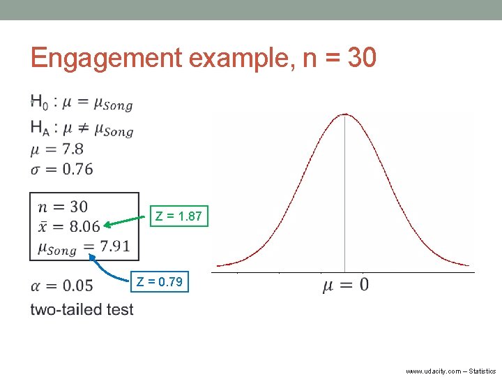
Engagement example, n = 30 • Z = 1. 87 Z = 0. 79 www. udacity. com – Statistics

Engagement example, n = 30 Which of these four quadrants represent the result of our hypothesis test? Decision Reject H 0 State of the world Retain H 0 true H 0 false www. udacity. com – Statistics

Engagement example, n = 30 Which of these four quadrants represent the result of our hypothesis test? Decision Reject H 0 State of the world H 0 true H 0 false Retain H 0 X

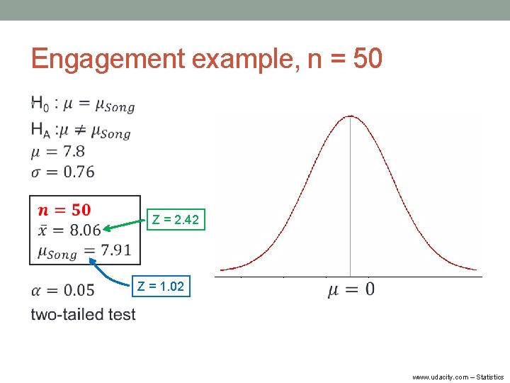
Engagement example, n = 50 • Z = 2. 42 Z = 1. 02 www. udacity. com – Statistics

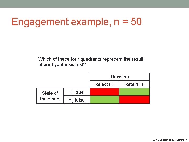
Engagement example, n = 50 Which of these four quadrants represent the result of our hypothesis test? Decision Reject H 0 State of the world Retain H 0 true H 0 false www. udacity. com – Statistics

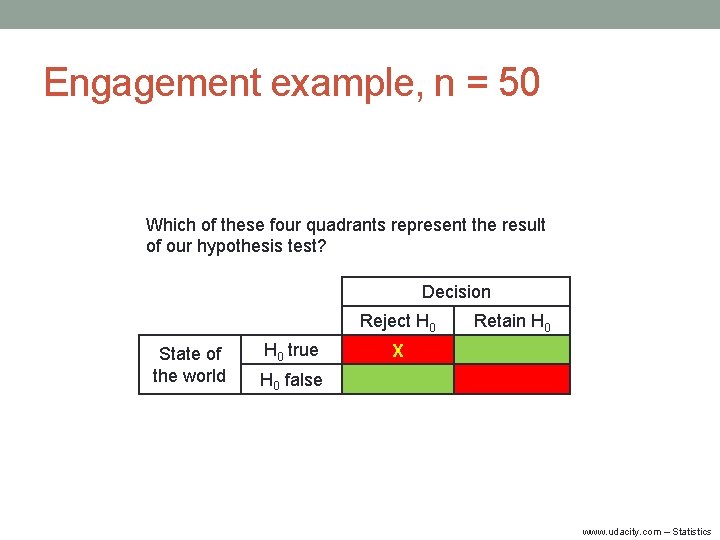
Engagement example, n = 50 Which of these four quadrants represent the result of our hypothesis test? Decision Reject H 0 State of the world H 0 true Retain H 0 X H 0 false www. udacity. com – Statistics

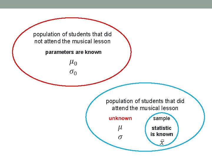
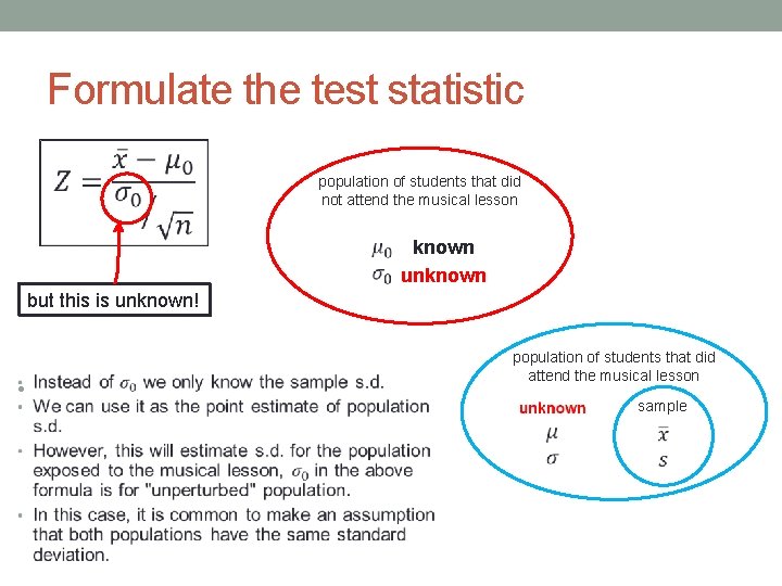
population of students that did not attend the musical lesson parameters are known population of students that did attend the musical lesson sample statistic is known

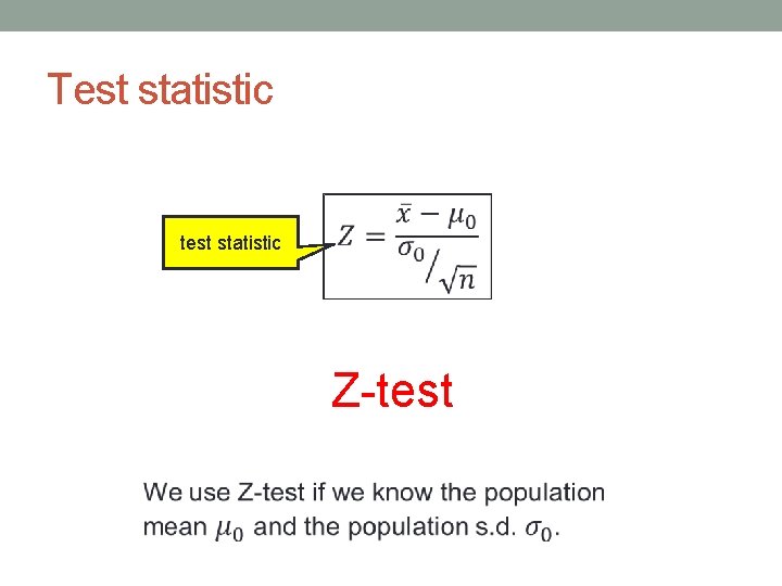
Test statistic test statistic Z-test

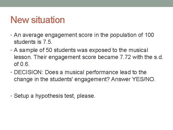
New situation • An average engagement score in the population of 100 students is 7. 5. • A sample of 50 students was exposed to the musical lesson. Their engagement score became 7. 72 with the s. d. of 0. 6. • DECISION: Does a musical performance lead to the change in the students' engagement? Answer YES/NO. • Setup a hypothesis test, please.

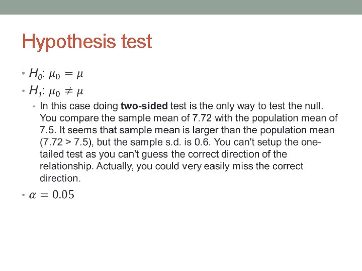
Hypothesis test •

Formulate the test statistic population of students that did not attend the musical lesson known unknown but this is unknown! • population of students that did attend the musical lesson sample

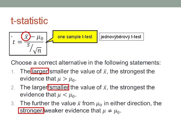
t-statistic • one sample t-test jednovýběrový t-test

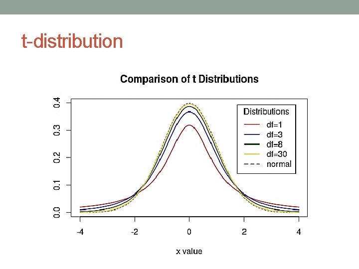
t-distribution

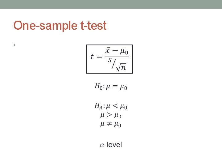
One-sample t-test •

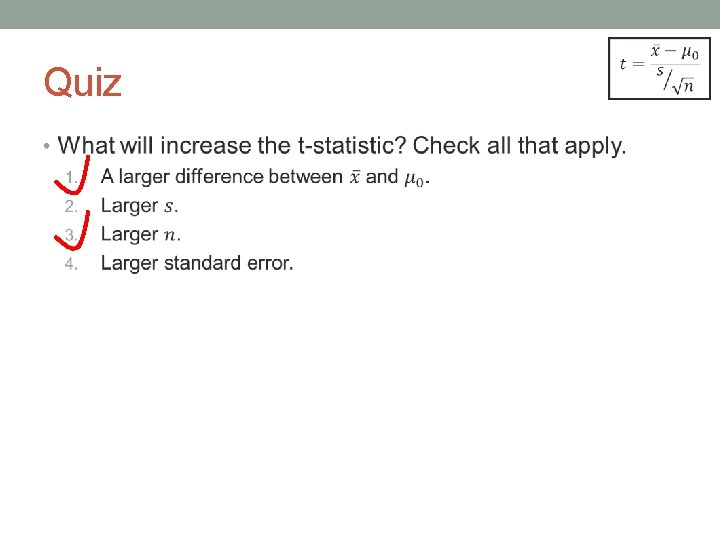
Quiz •

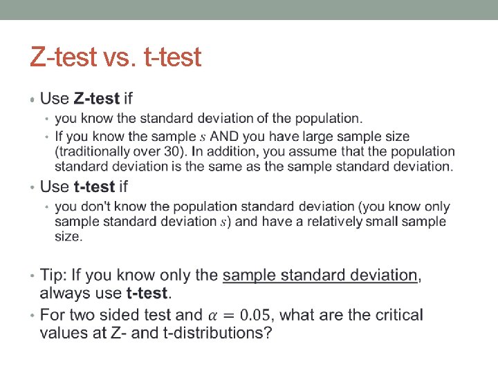
Z-test vs. t-test •

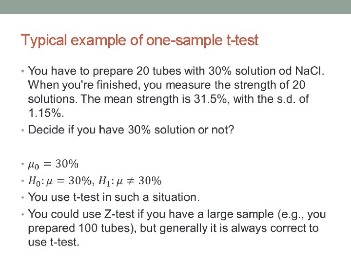
Typical example of one-sample t-test •

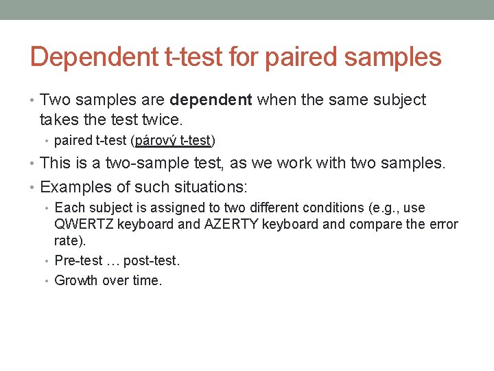
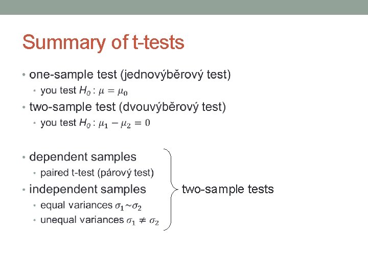
Dependent t-test for paired samples • Two samples are dependent when the same subject takes the test twice. • paired t-test (párový t-test) • This is a two-sample test, as we work with two samples. • Examples of such situations: • Each subject is assigned to two different conditions (e. g. , use QWERTZ keyboard and AZERTY keyboard and compare the error rate). • Pre-test … post-test. • Growth over time.

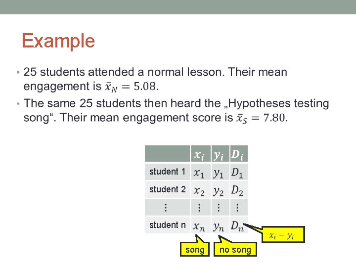
Example • student 1 student 2 student n song no song

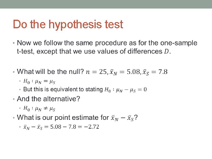
Do the hypothesis test •

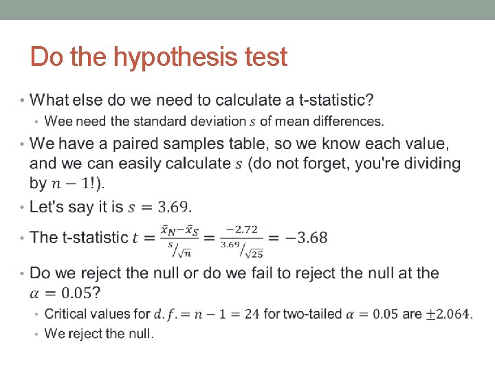
Do the hypothesis test •

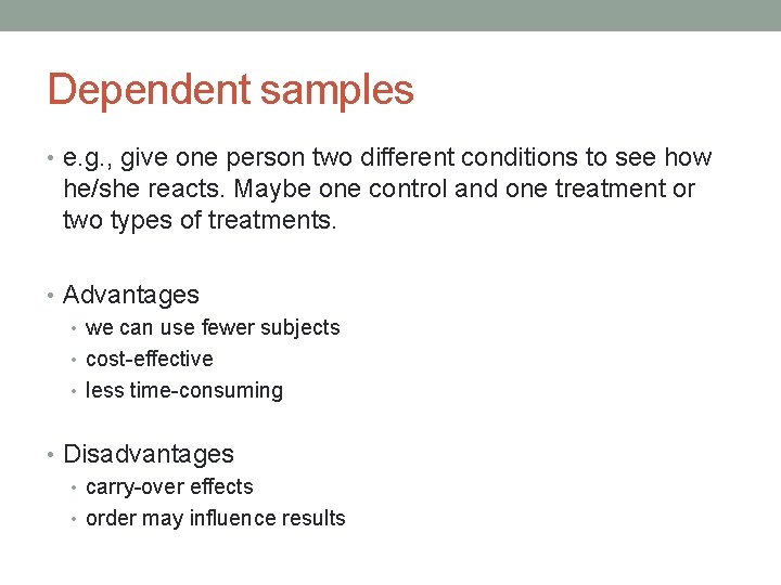
Dependent samples • e. g. , give one person two different conditions to see how he/she reacts. Maybe one control and one treatment or two types of treatments. • Advantages • we can use fewer subjects • cost-effective • less time-consuming • Disadvantages • carry-over effects • order may influence results

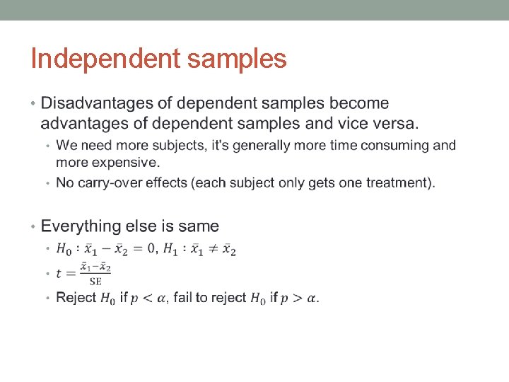
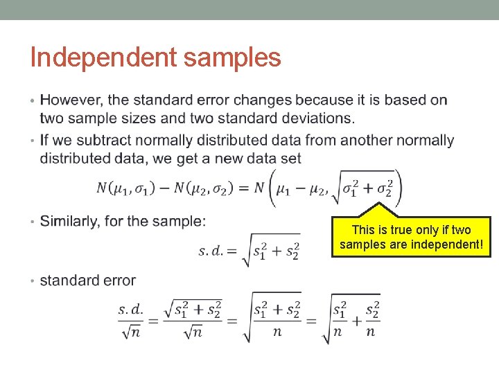
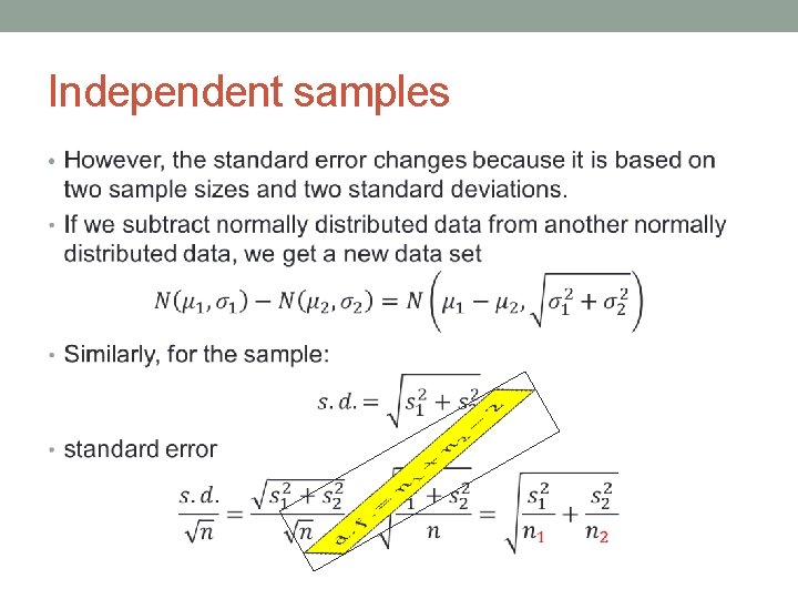
Independent samples •

Independent samples • This is true only if two samples are independent!

Independent samples •

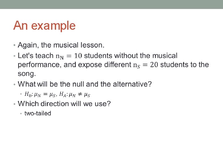
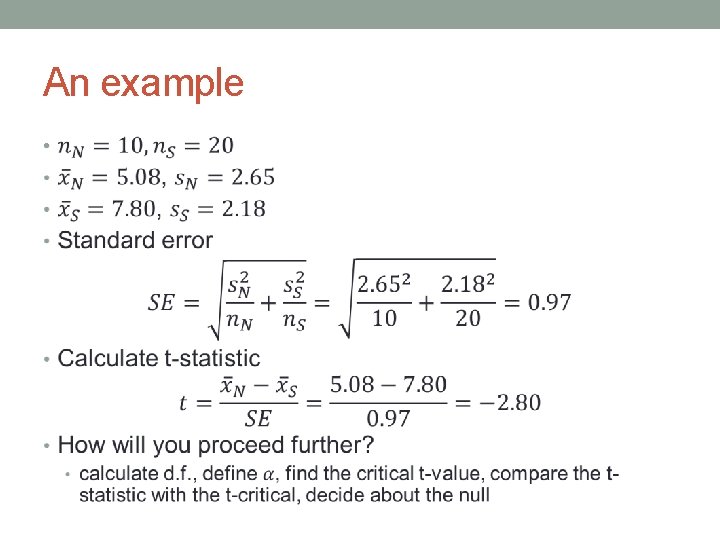
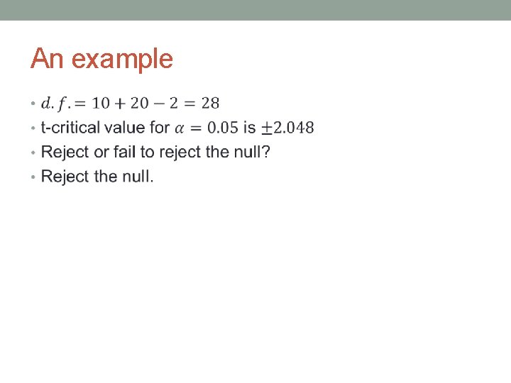
An example •

An example •

An example •

Summary of t-tests • two-sample tests

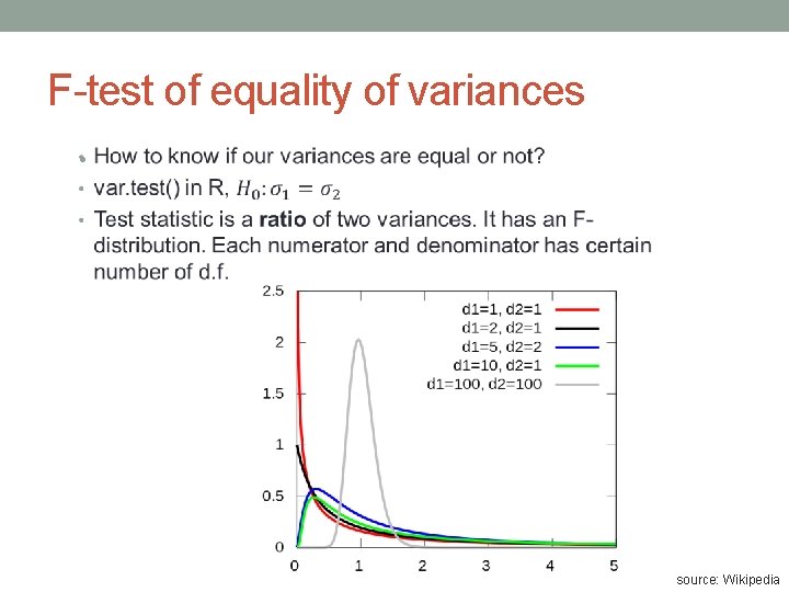
F-test of equality of variances • source: Wikipedia

t-test in R • t. test() • Let's have a look into R manual: http: //stat. ethz. ch/R-manual/R-patched/library/stats/html/t. test. html • See my website for link to pdf explaining various t-test in R (with examples).

Assumptions 1. Unpaired t-tests are highly sensitive to the violation of the independence assumption. 2. Populations samples come from should be approximately normal. • This is less important for large sample sizes. • What to do if these assumptions are not fullfilled 1. Use paired t-test 2. Let's see further

Check for normality – histogram

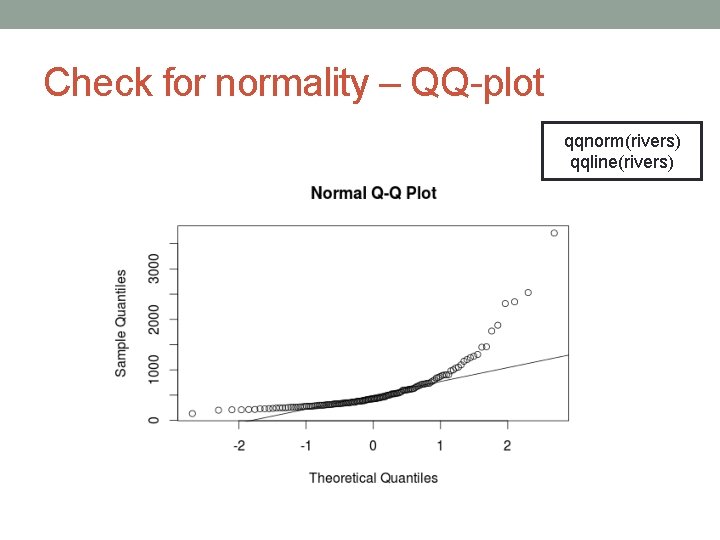
Check for normality – QQ-plot qqnorm(rivers) qqline(rivers)

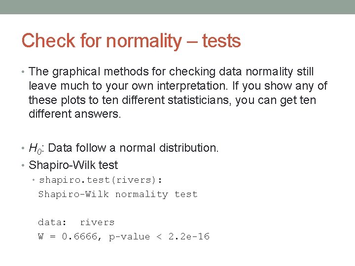
Check for normality – tests • The graphical methods for checking data normality still leave much to your own interpretation. If you show any of these plots to ten different statisticians, you can get ten different answers. • H 0: Data follow a normal distribution. • Shapiro-Wilk test • shapiro. test(rivers): Shapiro-Wilk normality test data: rivers W = 0. 6666, p-value < 2. 2 e-16

Nonparametric statistics • Small samples from considerably non-normal distributions. • non-parametric tests • No assumption about the shape of the distribution. • No assumption about the parameters of the distribution (thus they are called non-parametric). • Simple to do, however their theory is extremely complicated. Of course, we won't cover it at all. • However, they are less accurate than their parametric counterparts. • So if your data fullfill the assumptions about normality, use paramatric tests (t-test, F-test).

Nonparametric tests • If the normality assumption of the t-test is violated, and the sample sizes are too small, then its nonparametric alternative should be used. • The nonparametric alternative of t-test is Wilcoxon test. • wilcox. test() • http: //stat. ethz. ch/R-manual/R-patched/library/stats/html/wilcox. test. html