HYDROLOGY Lecture 2 ASSOC PROF DR TARK AN

HYDROLOGY Lecture 2 ASSOC. PROF. DR. TARK AN ERDIK

What is precipitation? • Precipitation is all forms of water that reach the surface from the atmosphere; it includes rain, snow, hail. All water enters the land in phase of the hydrologic cycle as precipitation. The hydrologists need to understand how the amount, rate, duration, and quality of precipitation are distributed in space and time:

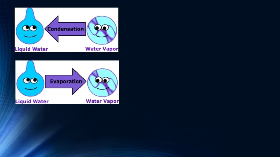
The Precipitation Process a sequence of four processes must occur: (1) Sufficient vapor should exist such that 90% of the precipitation comes from the water evaporated from oceans. (2) Air mass should be cooled. (3) Condensation must occur. Water condenses into liquid form when the saturation point is reached. (4) Drops that are sufficiently large (about 1 mm) should be formed.

Artificial rainfall (cloud seeding)

Types of precipitation Convective Precipitation Convective precipitation occurs when surface heating creates atmospheric instability that accelerates vertical uplift. Such precipitation is local, of short duration and heavy.

Cyclonic (frontal) precipitation Forward moving cold dense air causes the uplift of the warm lighter air in advance of the front. Because this uplift is relatively rapid along a steep frontal gradient, the condensed water vapor quickly organizes itself into heavy showers. Along the gently sloping warm front, the lifting of moist air produces precipitation that is less intense along this front, varying from moderate to light showers.

Orographic precipitation Winds carrying moisture from the sea rise up the windward side of the mountain. Once air cools, moisture condenses and precipitation falls on the windward side of the mountain. Positive correlation exist between the elevation and depth of precipitation.

Measurements Precipitation is the input to the land phase of the hydrologic cycle, so its accurate measurement is the essential foundation for quantitative hydrologic analyses, such as real-time flood forecasting or calibration and validation of hydrologic models Observations of precipitation are made as point measurements at traditional rain-gauge stations (section 4. 2. 1) and over areas via radar (section 4. 2. 2) and satellite (section 4. 2. 3). Observations of precipitation Non-recording (pluvyometer) Recording (pluvyograf) Rain gage stations Radar

Non-recording gauges

Conventional recording gauges Weighing gauges • Consists of a receiver bucket supported by a spring or lever balance or any other weighing mechanism. • The movement of bucket due to its increasing weight is transmitted to a pen which traces the record on a clock driven chart.

Tipping-bucket gauges Consists of 30 cm dia sharp edge receiver. At the end of it a funnel is provided. Under the funnel a pair of buckets are pivoted (the central point which balances). When the bucket receives 0. 25 mm of rainfall it tips, discharging its contents in the other bucket under funnel. Tipping of bucket completes an electric circuit causing movement of pen to mark on clock driven revolving drum which carries a record sheet.

Floating rain gauges It collects precipitation in a vessel containing a float that is connected to an analog or digital recording device. Precision depends on the float and recording mechanism.

Radar Measurement Ground-based radar can be used to estimate the areal distribution of instantaneous precipitation rates in clouds, and these rates can be electronically integrated to provide estimates of total precipitation for any time period. Energy of the reflected waves is proportional to the size of rainfal drops namely to the intensity of precipitation. Radars can be used for areal rainfall determination and should be calibrated by another raingauge on the ground.

Measurement of Snowfall measurements consist of snowfall and snow cover Snowfall is measured by gages used for rainfall. Non recording gages and weighing gages can be used. Antifreeze additives such as calcium chloride should be used. Gauges should be installed at a sufficient distance above the ground.

Snow cover measurements consist of 1 -Area covered by snow 2 -Thickness of snow 3 -Density of snow Measuring of snow depth should be performed on a 30× 30 cm white wooden board. Water equivalent of snow is the depth of water when the snow melts.

Measurement Errors Most precipitation gauges project above the ground surface and cause wind eddies that tend to reduce the catch, especially of smaller raindrops and snowflakes. Shapes of precipitation gauges used in various countries showing their effects on wind eddies that reduce gauge catches [courtesy of World Meteorological Organization (2008), Guide to Meteorological Instruments and Methods of Observation]. The errors can be around 10% and might be as large as 50% in light rainfall. Windscreens should be installed.

Alter type rainfall gauge (United States); Nipher type rainfall gauge(Canada) Tretyakov type rainfall gauge (Russia).

Important aspects of wind gauges. 1 -High obstacles such as trees and buildings might reduce rainfall drops entering the gauge. Gauges must be placed at a distance of at least two times the height of the obstacles. 2 -Evoporation of the water in the gauge must be prevented by forming thin layer oil on the water surface 3 -If the gauge is placed too high, the wind effect is stronger. On the other hand, if it is too low , raindrops that hit the ground may jump into the gauge.

Gauges network Gauges should be dense enough to determine areal distribution. Gauges must be placed denser in mountainous regions. Economical considerations may not allow a network that is as dense as desired WMO recommends one gauge per 600 -900 km 2 in plains and one gauge per 100 -250 km 2 in mountains regions. Interval of the elevations must be less than 500 m. At least 10 and 20% of the gauges should be recording type.

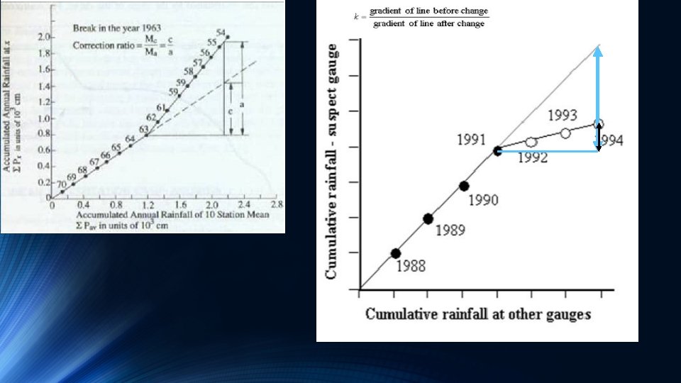
Double-mass curve (A common technique for detecting and correcting for inconsistent precipitation data) A double-mass curve is a plot, on arithmetic graph paper, of the successive cumulative annual precipitation collected at a gauge where measurement conditions may have changed significantly versus the successive cumulative average of the annual precipitation. The method attempts to detect a change in the proportionality between the measurements at the suspect station and those of the region.

Year A (mm) B (mm) C (mm) D (mm) E (mm) 1976 1977 1, 010 1, 005 1, 161 978 780 1, 041 949 784 834 713 1978 1, 067 1, 226 1, 027 1, 067 851 1979 1, 051 880 825 1, 014 751 1980 801 1, 146 933 923 604 1981 1, 411 1, 353 1, 584 930 1, 483 1982 1, 222 1, 018 1, 215 981 1, 174 1983 1, 012 751 832 683 771 1984 1, 153 1, 059 918 824 1, 188 1985 1, 140 1, 223 781 1, 056 967 1986 829 1, 003 899 796 1, 088 1987 1, 165 1, 120 995 1, 121 963 1988 1, 170 989 1, 099 1, 286 1, 287 1989 1, 264 1, 056 1, 266 1, 044 1, 190 1990 1, 200 1, 261 1, 216 991 1, 283 1991 942 811 817 875 873 1992 1, 166 969 1, 331 1, 202 1, 209 Station under suspicion

Precipitation Mass Curve and Hyetograph Mass curve: A record of precipitation depth as a function of time. 10 Cumulative Rainfall (cm) 9 8 7 6 5 4 3 2 1 0 0 30 60 Time (min. ) 90 120 150

Example: Rainfall values of a certain precipitation is given below. Please calculate mass curve with time. Time (min) Rainfall (cm) 0 5 10 15 20 25 30 35 40 45 0 0. 2 3. 4 1 0. 4 1. 9 4. 8 5 5 5. 1

0 5 10 15 20 25 30 35 40 45 0 0. 2 3. 4 1 0. 4 1. 9 4. 8 5 5 5. 1 0 0. 2 3. 6 4. 6 5 6. 9 11. 7 16. 7 21. 7 26. 8 Cumulative Rainfall (cm) 30 25 20 P (cm) Time (min) Cumulative Rainfall (cm) 15 10 5 0 0 5 10 15 20 25 t (min) 30 35 40 45 50

Rainfall intensity: Amount of rain that falls to the earth surface per unit of time 10 9 Cumulative Rainfall (cm) 8 7 6 5 4 8. 2 cm 3 5. 56 cm 2 1 1 hr 2 hr 0 0 30 60 Time (min. ) 90 120 150

Example Time, t (min) Accumulated rainfall (P, cm) ∆P (cm) 5 0. 1 10 0. 2 15 0. 8 20 1. 5 25 1. 8 30 2 35 2. 5 40 2. 7 45 2. 9 50 3. 1 ∆t (sec) Intensity (cm/hour)

Time, t (min) Accumulated rainfall (P, cm) ∆P (cm) ∆t (sec) Intensity (cm/hour) 5 0. 1 5 0. 02 1. 2 10 0. 2 0. 1 5 0. 02 1. 2 15 0. 8 0. 6 5 0. 12 7. 2 20 1. 5 0. 7 5 0. 14 8. 4 25 1. 8 0. 3 5 0. 06 3. 6 30 2 0. 2 5 0. 04 2. 4 35 2. 5 0. 5 5 0. 1 6 40 2. 7 0. 2 5 0. 04 2. 4 45 2. 9 0. 2 5 0. 04 2. 4 50 3. 1 0. 2 5 0. 04 2. 4

Hyetograph: Variation of precipitation or namely intensity with time. Total precipitation is the area beneath the curve= (1. 2× 10+7. 2× 5+8. 4× 5+3. 6× 5+2. 4× 5+6× 5+2. 4× 15)=186 cm×min/hr=3. 1 cm

Arithmetic Mean Method • Simplest method for determining areal average P 1 = 10 mm P 1 P 2 = 20 mm P 3 = 30 mm P 2 P 3 • Gages must be uniformly distributed • Gage measurements should not vary greatly about the mean

Thiessen polygon method • • • Any point in the watershed receives the same amount of rainfall as that at the nearest gage Rainfall recorded at a gage can be applied to any point at a distance halfway to the next station in any direction P 1 A 1 P 2 Steps in Thiessen polygon method A 2 1. Draw lines joining adjacent gages P 3 2. Draw perpendicular bisectors to the lines created in step 1 A 3 3. Extend the lines created in step 2 in both directions to form representative areas for gages 4. Compute representative area for each gage 5. Compute the areal average using the following formula P 1 = 10 mm, A 1 = 12 Km 2 P 2 = 20 mm, A 2 = 15 Km 2 P 3 = 30 mm, A 3 = 20 2

Isohyetal method • Steps • Construct isohyets (rainfall contours) • Compute area between each pair of adjacent isohyets (Ai) • Compute average precipitation for each pair of adjacent isohyets (pi) 10 20 P 1 A 1=5 , p 1 = 5 A 2=18 , p 2 = 15 P 2 A 3=12 , p 3 = 25 • Compute areal average using the following formula 30 P 3 A 4=12 , p 3 = 35