HYDROLOGY Lecture 11 IUH ASSOC PROF DR TARK

HYDROLOGY Lecture 11 IUH ASSOC. PROF. DR. TARK AN ERDIK

Instantaneous Unit Hydrograph: Instantaneous unit hydrograph (IUH) is obtained when the duration of the rainfall excess is infinitesimally small. Why do we need IUH? Because some basic assumptions below of Unit Hydrograph Theory is violated. 1 -Large areas, areas more than 5000 km square unit hydrograph approach will not be valid. 2 - Actual rainfall event may not follow a uniform intensity for a large period of time. In those cases above, rainfall will not be uniform so IUH should be used.

i Unit Hydrograph What would happen if we reduce D to D/2 intensity will be increased to 2 i What would happen if we reduce D to D/4 intensity will be increased to 4 i What would happen if we reduce D to 0 intensity will be increased to infinity We can reduce the duration to 0 and that is why this is called an instantaneous unit hydrograph. The intensity is infinite, of course, the duration is 0.

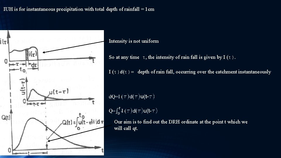
IUH is for instantaneous precipitation with total depth of rainfall = 1 cm Intensity is not uniform So at any time τ, the intensity of rain fall is given by I (τ)d(τ)= depth of rain fall, occurring over the catchment instantaneously Our aim is to find out the DRH ordinate at the point t which we will call qt.

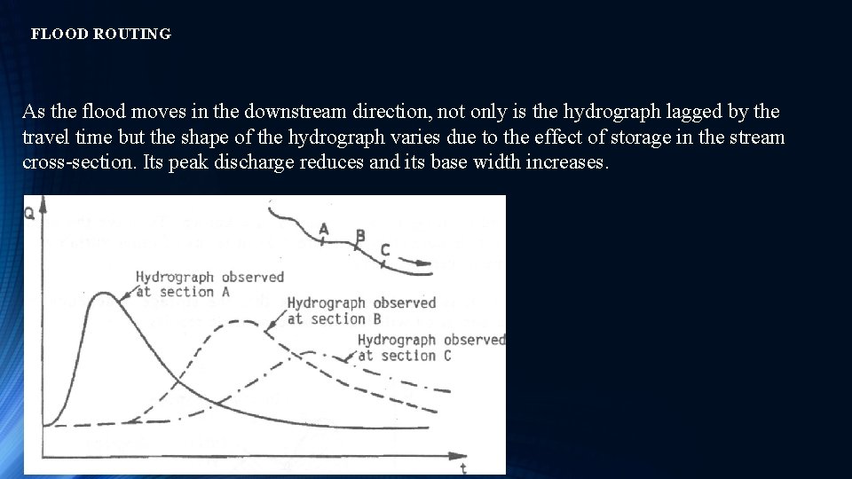
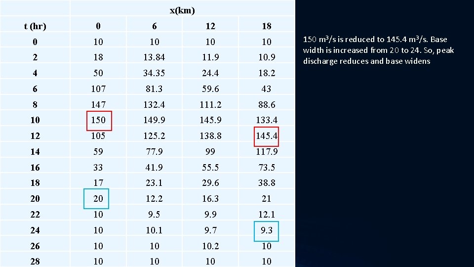
FLOOD ROUTING As the flood moves in the downstream direction, not only is the hydrograph lagged by the travel time but the shape of the hydrograph varies due to the effect of storage in the stream cross-section. Its peak discharge reduces and its base width increases.

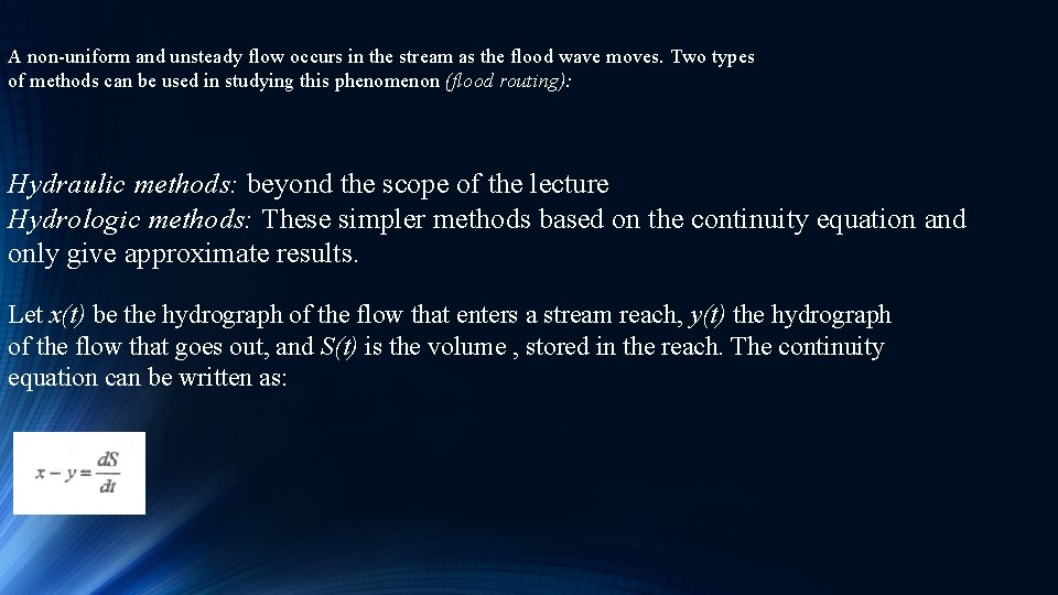
A non-uniform and unsteady flow occurs in the stream as the flood wave moves. Two types of methods can be used in studying this phenomenon (flood routing): Hydraulic methods: beyond the scope of the lecture Hydrologic methods: These simpler methods based on the continuity equation and only give approximate results. Let x(t) be the hydrograph of the flow that enters a stream reach, y(t) the hydrograph of the flow that goes out, and S(t) is the volume , stored in the reach. The continuity equation can be written as:

In flood routing, x 1, x 2, y 1, and S 1 are known. To solve the unknowns S 2 and y 2, it is necessary to express S 2 in terms of other variables.

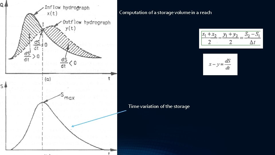
Computation of a storage volume in a reach Time variation of the storage

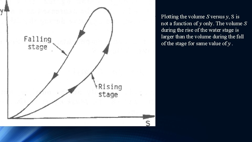
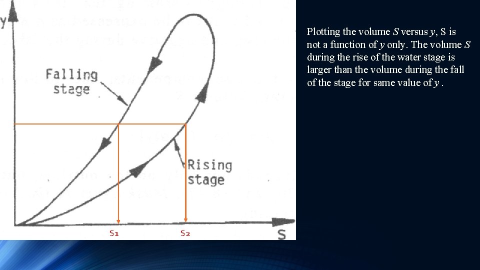
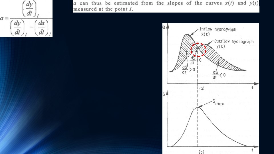
Plotting the volume S versus y, S is not a function of y only. The volume S during the rise of the water stage is larger than the volume during the fall of the stage for same value of y.

Plotting the volume S versus y, S is not a function of y only. The volume S during the rise of the water stage is larger than the volume during the fall of the stage for same value of y. S 1 S 2

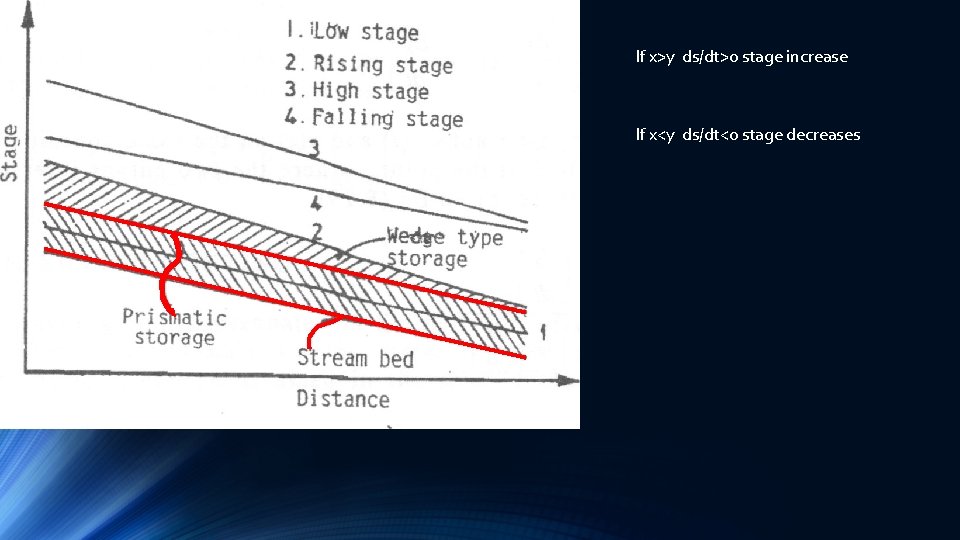
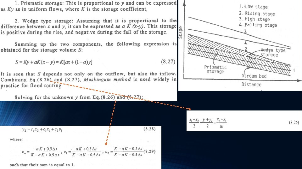
If x>y ds/dt>0 stage increase If x<y ds/dt<0 stage decreases

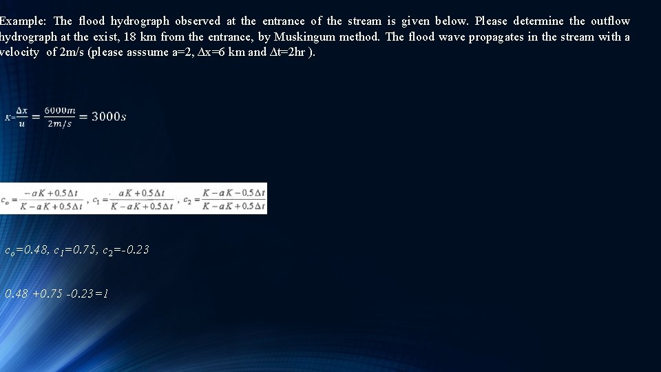
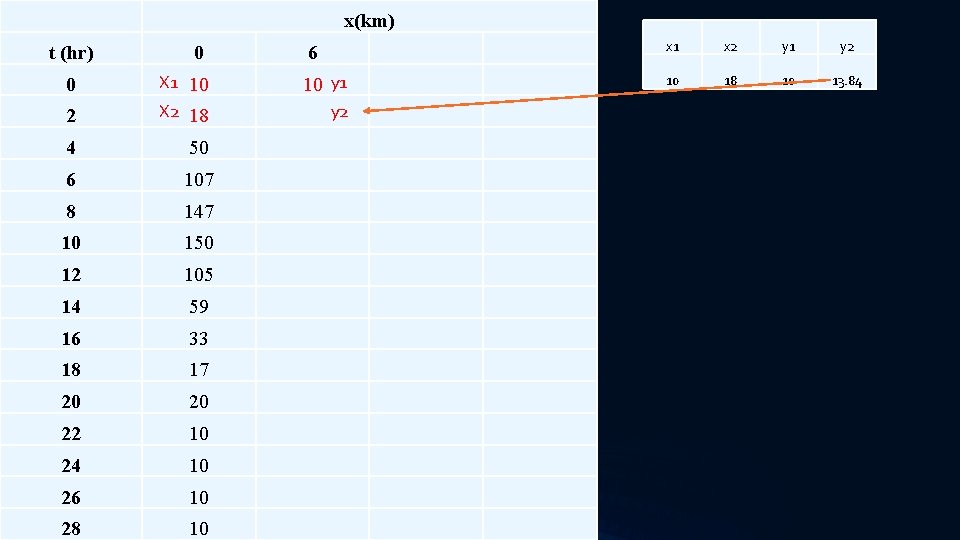
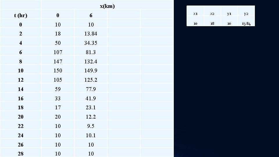
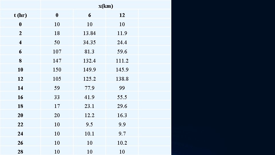
Example: The flood hydrograph observed at the entrance of the stream is given below. Please determine the outflow hydrograph at the exist, 18 km from the entrance, by Muskingum method. The flood wave propagates in the stream with a velocity of 2 m/s (please asssume a=2, ∆x=6 km and ∆t=2 hr ). co =0. 48, c 1 =0. 75, c 2 =-0. 23 0. 48 +0. 75 -0. 23=1

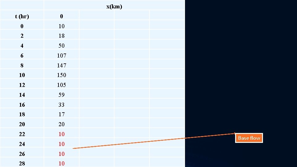
x(km) t (hr) 0 0 10 2 18 4 50 6 107 8 147 10 150 12 105 14 59 16 33 18 17 20 20 22 10 24 10 26 10 28 10 Base flow

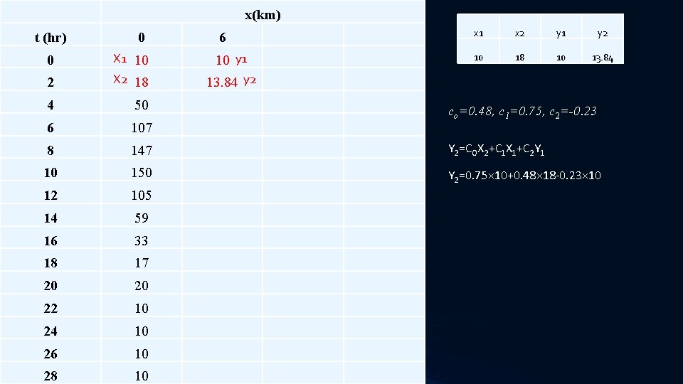
x(km) t (hr) 0 6 x 2 y 1 y 2 10 18 10 13. 84 2 X 1 10 X 2 18 4 50 6 107 8 147 Y 2=COX 2+C 1 X 1+C 2 Y 1 10 150 Y 2=0. 75× 10+0. 48× 18 -0. 23× 10 12 105 14 59 16 33 18 17 20 20 22 10 24 10 26 10 28 10 0 10 y 1 x 1 13. 84 y 2 co =0. 48, c 1 =0. 75, c 2 =-0. 23

x(km) t (hr) 0 2 X 1 10 X 2 18 4 50 6 107 8 147 10 150 12 105 14 59 16 33 18 17 20 20 22 10 24 10 26 10 28 10 0 6 10 y 1 y 2 x 1 x 2 y 1 y 2 10 18 10 13. 84

x(km) t (hr) 0 6 x 1 x 2 y 1 y 2 0 10 18 10 13. 84 2 18 13. 84 4 50 34. 35 6 107 81. 3 8 147 132. 4 10 150 149. 9 12 105 125. 2 14 59 77. 9 16 33 41. 9 18 17 23. 1 20 20 12. 2 22 10 9. 5 24 10 10. 1 26 10 10 28 10 10

x(km) t (hr) 0 6 12 0 10 10 10 2 18 13. 84 11. 9 4 50 34. 35 24. 4 6 107 81. 3 59. 6 8 147 132. 4 111. 2 10 150 149. 9 145. 9 12 105 125. 2 138. 8 14 59 77. 9 99 16 33 41. 9 55. 5 18 17 23. 1 29. 6 20 20 12. 2 16. 3 22 10 9. 5 9. 9 24 10 10. 1 9. 7 26 10 10 10. 2 28 10 10 10

x(km) t (hr) 0 6 12 18 0 10 10 2 18 13. 84 11. 9 10. 9 4 50 34. 35 24. 4 18. 2 6 107 81. 3 59. 6 43 8 147 132. 4 111. 2 88. 6 10 150 149. 9 145. 9 133. 4 12 105 125. 2 138. 8 145. 4 14 59 77. 9 99 117. 9 16 33 41. 9 55. 5 73. 5 18 17 23. 1 29. 6 38. 8 20 20 12. 2 16. 3 21 22 10 9. 5 9. 9 12. 1 24 10 10. 1 9. 7 9. 3 26 10 10 10. 2 10 28 10 10 150 m 3/s is reduced to 145. 4 m 3/s. Base width is increased from 20 to 24. So, peak discharge reduces and base widens