Honours Finance Advanced Topics in Finance Nonlinear Analysis

Honours Finance (Advanced Topics in Finance: Nonlinear Analysis) Lecture 3: Introduction to ODEs continued

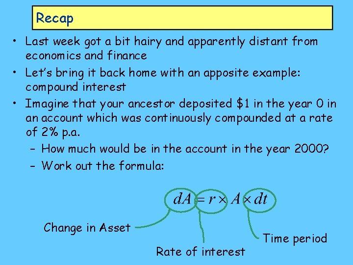
Recap • Last week got a bit hairy and apparently distant from economics and finance • Let’s bring it back home with an apposite example: compound interest • Imagine that your ancestor deposited $1 in the year 0 in an account which was continuously compounded at a rate of 2% p. a. – How much would be in the account in the year 2000? – Work out the formula: Change in Asset Rate of interest Time period

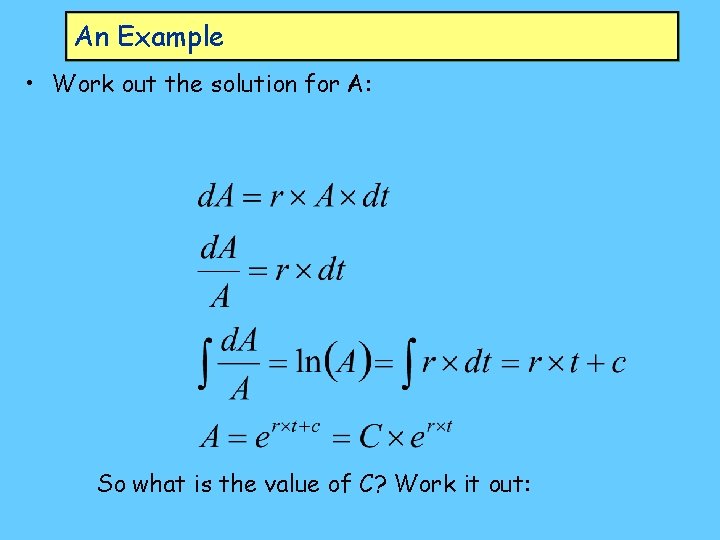
An Example • Work out the solution for A: So what is the value of C? Work it out:

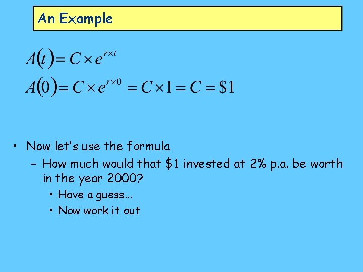
An Example • Now let’s use the formula – How much would that $1 invested at 2% p. a. be worth in the year 2000? • Have a guess. . . • Now work it out

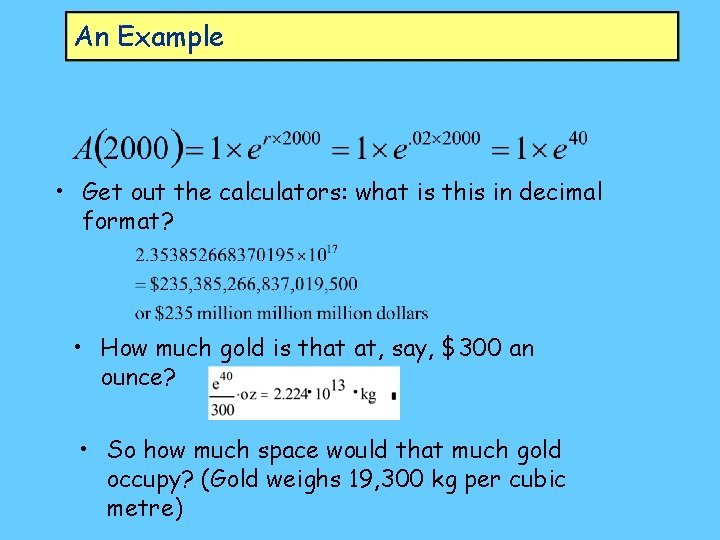
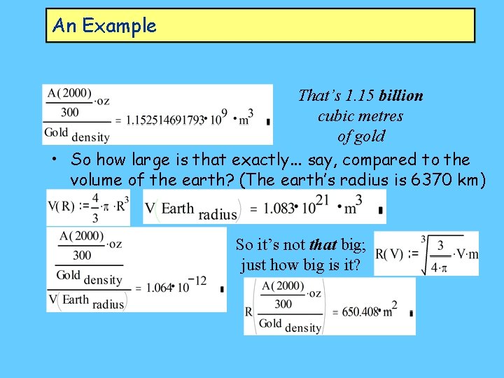
An Example • Get out the calculators: what is this in decimal format? • How much gold is that at, say, $300 an ounce? • So how much space would that much gold occupy? (Gold weighs 19, 300 kg per cubic metre)

An Example That’s 1. 15 billion cubic metres of gold • So how large is that exactly. . . say, compared to the volume of the earth? (The earth’s radius is 6370 km) So it’s not that big; just how big is it?

An Example • So one dollar, invested at 2% p. a. , turns into a ball of gold 1300 metres across in 2000 years • And I bet you thought 2% was a lousy rate of return! • What do you think 4% yields? – 250, 000 balls of gold the size of the earth, or a sphere of gold 400, 000 km across! • With the knowledge imparted by this ODE, you should now be sceptical about the long term viability of growth rates which are currently taken as desirable in the modern world – 10% p. a. for China, etc. – World history hasn’t been one of continuous accumulation! – Current expected yields (4 -6% p. a. min. ) unsustainable…

Back to Solutions to ODEs • This week we’ll consider how to solve – first order separable nonlinear ODEs – second order linear ODEs • As a prelude to – systems of ODEs and complexity – chaotic behaviour in deterministic systems • (our real interest in a course on economics and finance) • But before considering more solution techniques, a reminder: – most ODEs are insoluble: impossible to find a closed form for y(t) from an expression for y’(t):

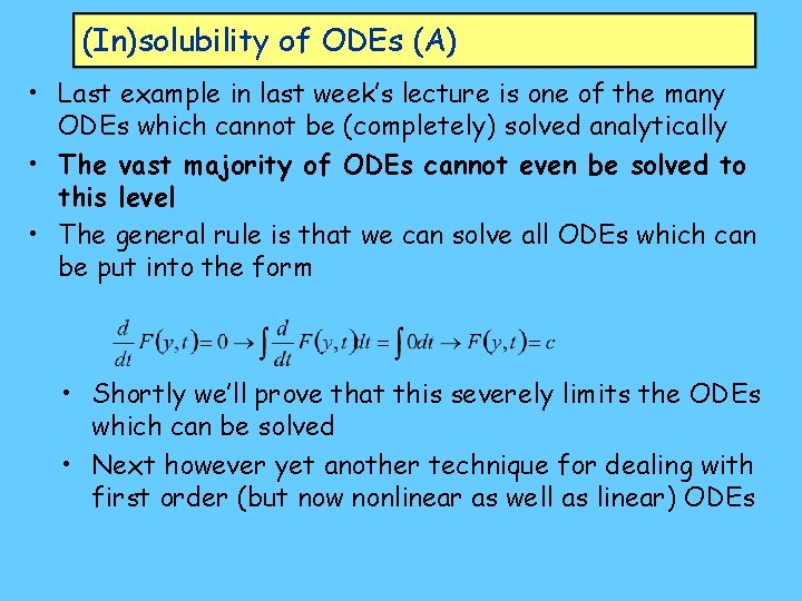
(In)solubility of ODEs (A) • Last example in last week’s lecture is one of the many ODEs which cannot be (completely) solved analytically • The vast majority of ODEs cannot even be solved to this level • The general rule is that we can solve all ODEs which can be put into the form • Shortly we’ll prove that this severely limits the ODEs which can be solved • Next however yet another technique for dealing with first order (but now nonlinear as well as linear) ODEs

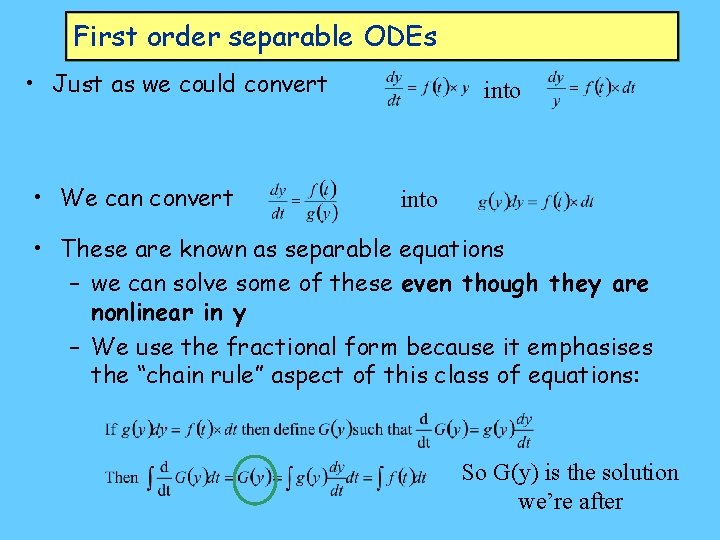
First order separable ODEs • Just as we could convert • We can convert into • These are known as separable equations – we can solve some of these even though they are nonlinear in y – We use the fractional form because it emphasises the “chain rule” aspect of this class of equations: So G(y) is the solution we’re after

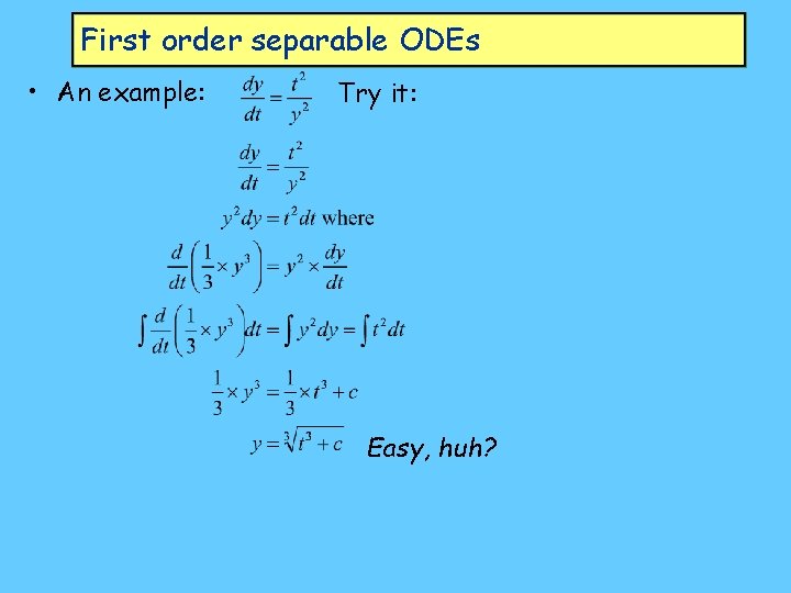
First order separable ODEs • An example: Try it: Easy, huh?

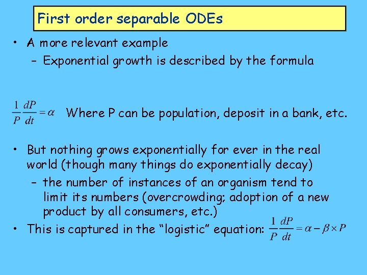
First order separable ODEs • A more relevant example – Exponential growth is described by the formula Where P can be population, deposit in a bank, etc. • But nothing grows exponentially for ever in the real world (though many things do exponentially decay) – the number of instances of an organism tend to limit its numbers (overcrowding; adoption of a new product by all consumers, etc. ) • This is captured in the “logistic” equation:

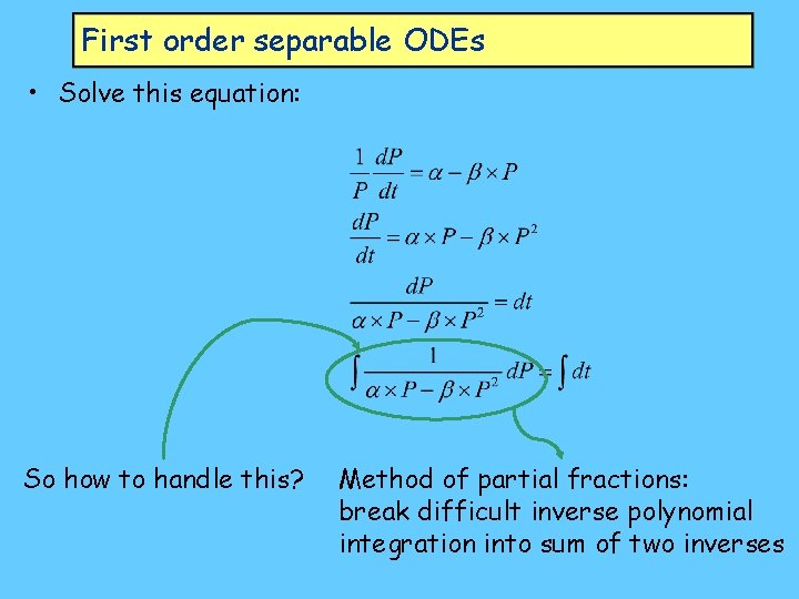
First order separable ODEs • Solve this equation: So how to handle this? Method of partial fractions: break difficult inverse polynomial integration into sum of two inverses

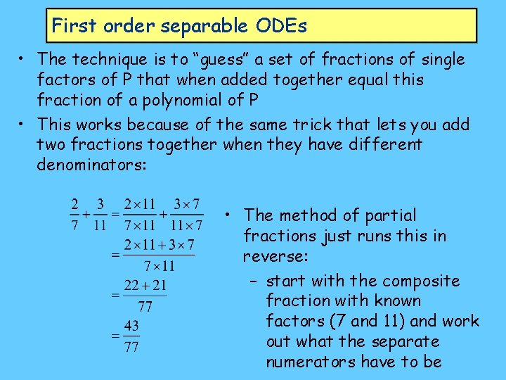
First order separable ODEs • The technique is to “guess” a set of fractions of single factors of P that when added together equal this fraction of a polynomial of P • This works because of the same trick that lets you add two fractions together when they have different denominators: • The method of partial fractions just runs this in reverse: – start with the composite fraction with known factors (7 and 11) and work out what the separate numerators have to be

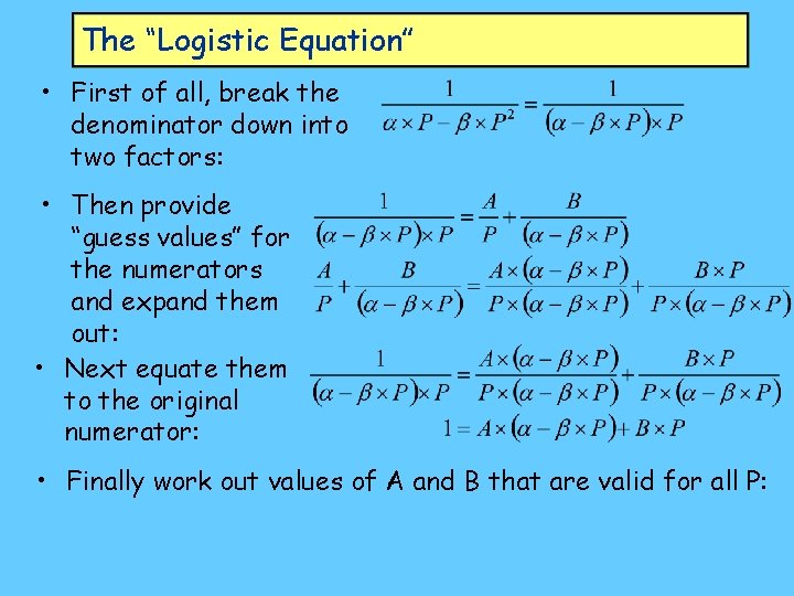
The “Logistic Equation” • First of all, break the denominator down into two factors: • Then provide “guess values” for the numerators and expand them out: • Next equate them to the original numerator: • Finally work out values of A and B that are valid for all P:

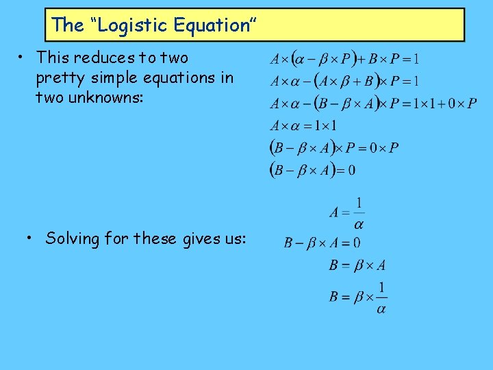
The “Logistic Equation” • This reduces to two pretty simple equations in two unknowns: • Solving for these gives us:

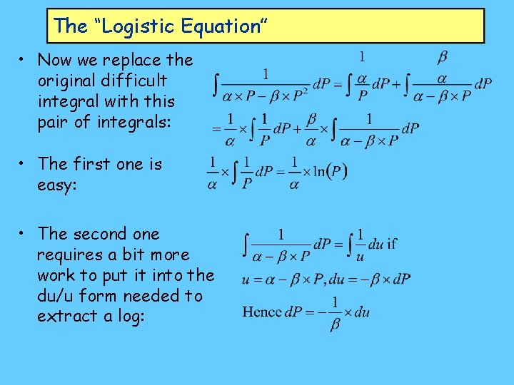
The “Logistic Equation” • Now we replace the original difficult integral with this pair of integrals: • The first one is easy: • The second one requires a bit more work to put it into the du/u form needed to extract a log:

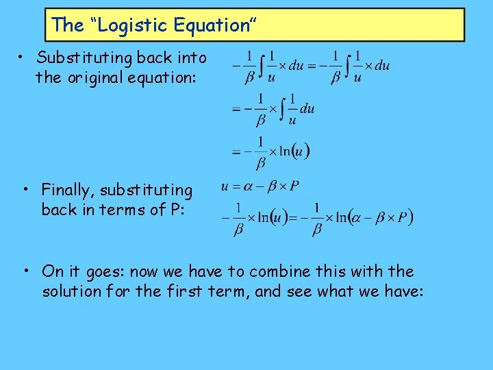
The “Logistic Equation” • Substituting back into the original equation: • Finally, substituting back in terms of P: • On it goes: now we have to combine this with the solution for the first term, and see what we have:

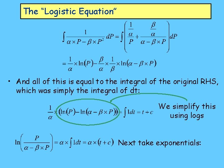
The “Logistic Equation” • And all of this is equal to the integral of the original RHS, which was simply the integral of dt: We simplify this using logs Next take exponentials:

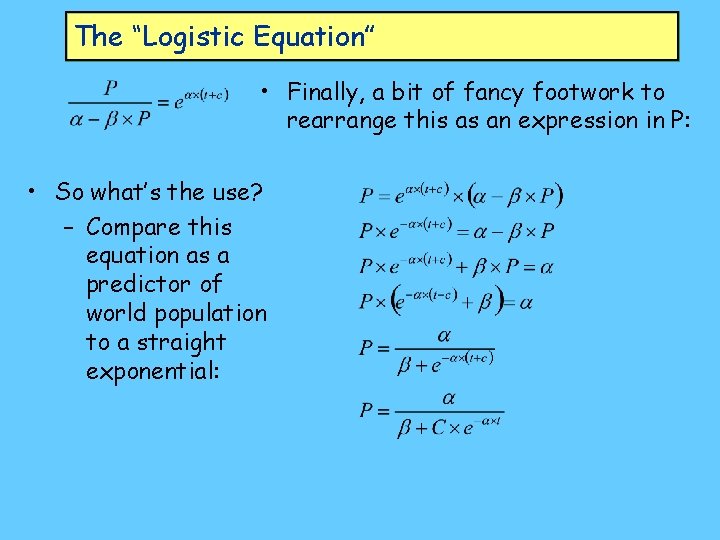
The “Logistic Equation” • Finally, a bit of fancy footwork to rearrange this as an expression in P: • So what’s the use? – Compare this equation as a predictor of world population to a straight exponential:

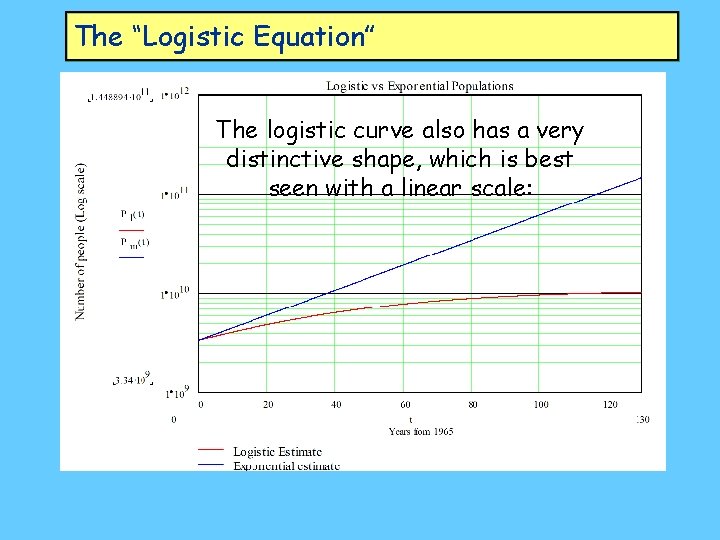
The “Logistic Equation” • Ecological estimates for a [(births-deaths)/population] give a value of 0. 029 (Braun 1993: 31) • When world population was 3. 34 billion in 1965, it was growing at 2% p. a. – We can put these values into the equation for P: • Now let’s compare a simple Malthusian estimate of population in the year 2100 with a logistic estimate, given a population of 3. 34 billion in 1965:

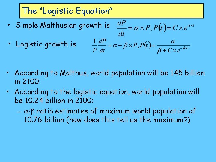
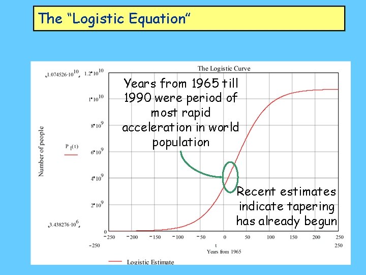
The “Logistic Equation” • Simple Malthusian growth is • Logistic growth is • According to Malthus, world population will be 145 billion in 2100 • According to the logistic equation, world population will be 10. 24 billion in 2100: – a/b ratio estimates of maximum world population of 10. 76 billion (how does this tell us the maximum? )

The “Logistic Equation” The logistic curve also has a very distinctive shape, which is best seen with a linear scale:

The “Logistic Equation” Years from 1965 till 1990 were period of most rapid acceleration in world population Recent estimates indicate tapering has already begun

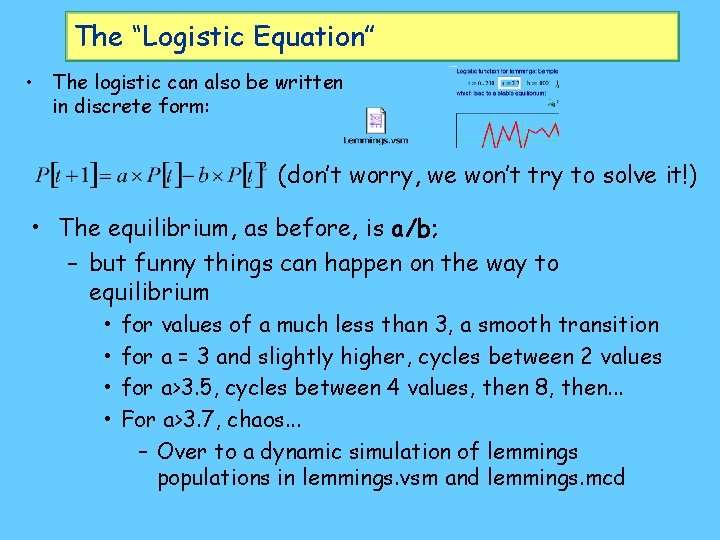
The “Logistic Equation” • The logistic can also be written in discrete form: (don’t worry, we won’t try to solve it!) • The equilibrium, as before, is a/b; – but funny things can happen on the way to equilibrium • • for values of a much less than 3, a smooth transition for a = 3 and slightly higher, cycles between 2 values for a>3. 5, cycles between 4 values, then 8, then. . . For a>3. 7, chaos. . . – Over to a dynamic simulation of lemmings populations in lemmings. vsm and lemmings. mcd

The “Logistic Equation” • Interpretation? – Low growth rates, population smoothly tapers to equilibrium – Higher growth rates, population overshoots • medium-high values, overshoot is cyclical – first a 2 -cycle, then a 4 -cycle • “equilibrium” is a 1 -cycle; higher order cycles are quite possible – eventually an infinite-cycle for values around 3. 7, then chaos • Aperiodic cycles: always fluctuates but fluctuations never repeat scale or period • apparent randomness from a deterministic process

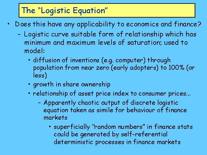
The “Logistic Equation” • Does this have any applicability to economics and finance? – Logistic curve suitable form of relationship which has minimum and maximum levels of saturation; used to model: • diffusion of inventions (e. g. computer) through population from near zero (early adopters) to 100% (or less) • growth in share ownership • relationship of asset price index to consumer prices. . . – Apparently chaotic output of discrete logistic equation taken as simile for behaviour of finance markets • superficially “random numbers” in finance stats could be generated by self-referential deterministic processes in finance markets

Back to ODEs in general • Clear role of differential/difference equations in economics and finance • Most such models sufficiently complex that can’t be solved at all • But to appreciate them, need to know how to solve the solvable ones. • However, we can prove that most ODEs can’t be solved!:

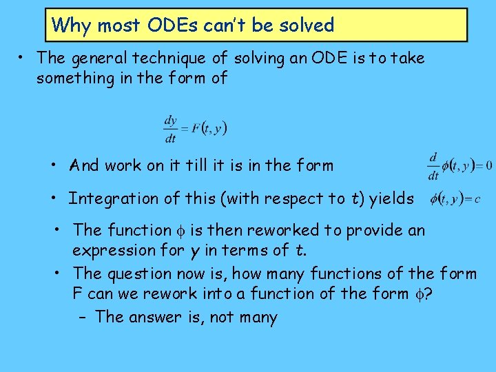
Why most ODEs can’t be solved • The general technique of solving an ODE is to take something in the form of • And work on it till it is in the form • Integration of this (with respect to t) yields • The function f is then reworked to provide an expression for y in terms of t. • The question now is, how many functions of the form F can we rework into a function of the form f? – The answer is, not many

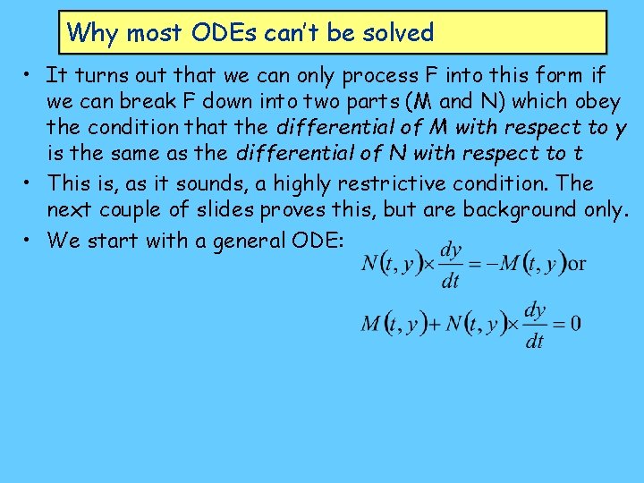
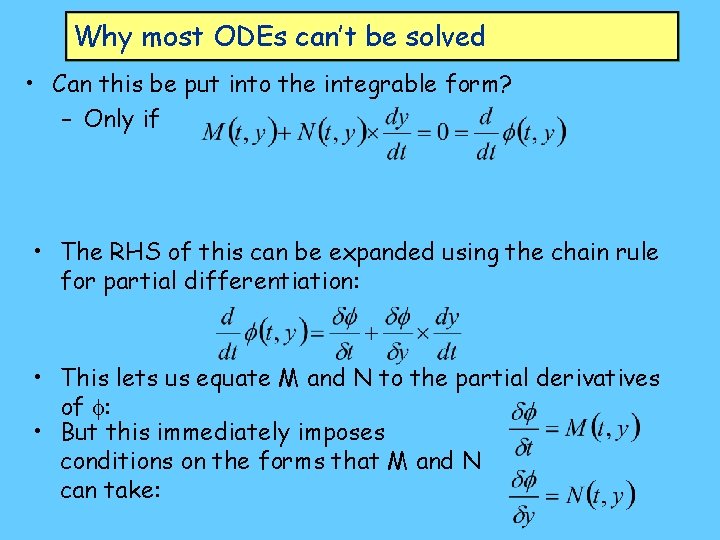
Why most ODEs can’t be solved • It turns out that we can only process F into this form if we can break F down into two parts (M and N) which obey the condition that the differential of M with respect to y is the same as the differential of N with respect to t • This is, as it sounds, a highly restrictive condition. The next couple of slides proves this, but are background only. • We start with a general ODE:

Why most ODEs can’t be solved • Can this be put into the integrable form? – Only if • The RHS of this can be expanded using the chain rule for partial differentiation: • This lets us equate M and N to the partial derivatives of f: • But this immediately imposes conditions on the forms that M and N can take:

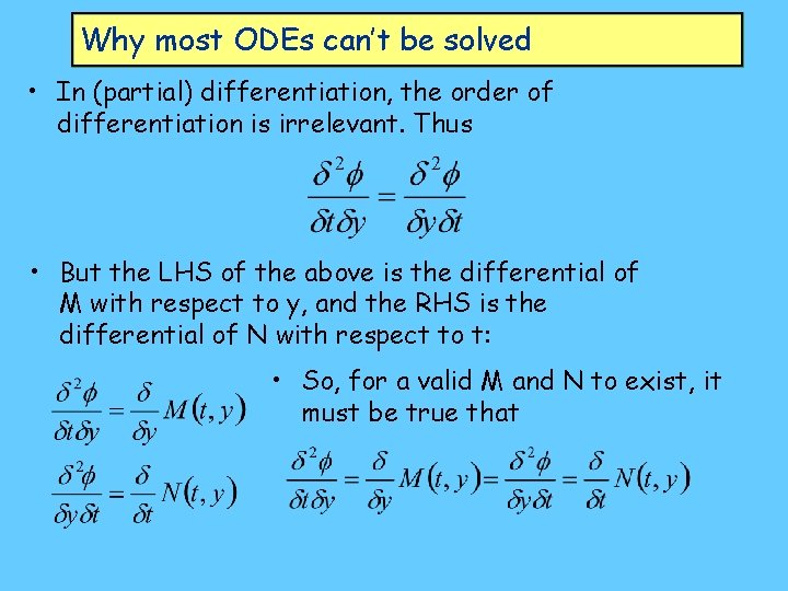
Why most ODEs can’t be solved • In (partial) differentiation, the order of differentiation is irrelevant. Thus • But the LHS of the above is the differential of M with respect to y, and the RHS is the differential of N with respect to t: • So, for a valid M and N to exist, it must be true that

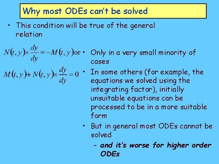
Why most ODEs can’t be solved • This condition will be true of the general relation • Only in a very small minority of cases • In some others (for example, the equations we solved using the integrating factor), initially unsuitable equations can be processed to be in a more suitable form • But in general most ODEs cannot be solved – and it’s worse for higher order ODEs

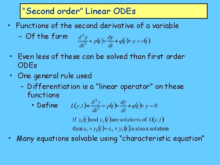
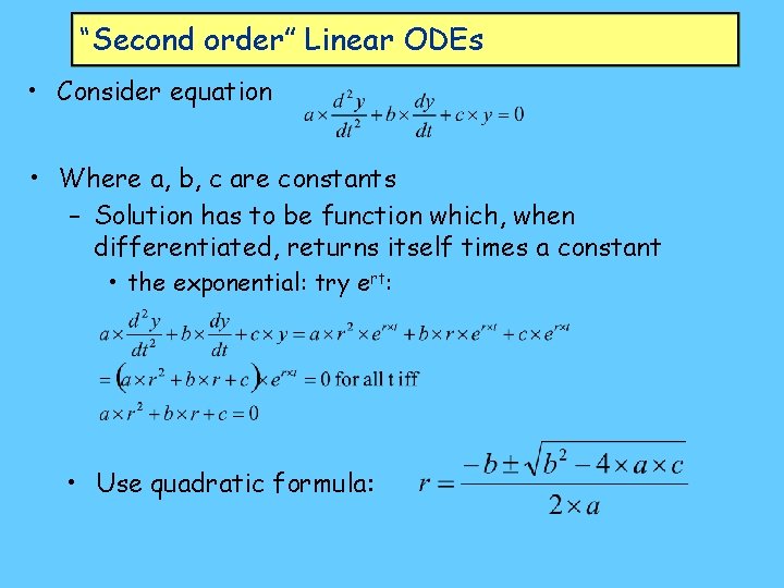
“Second order” Linear ODEs • Functions of the second derivative of a variable – Of the form • Even less of these can be solved than first order ODEs • One general rule used – Differentiation is a “linear operator” on these functions • Define • Many equations solvable using “characteristic equation”

“Second order” Linear ODEs • Consider equation • Where a, b, c are constants – Solution has to be function which, when differentiated, returns itself times a constant • the exponential: try ert: • Use quadratic formula:

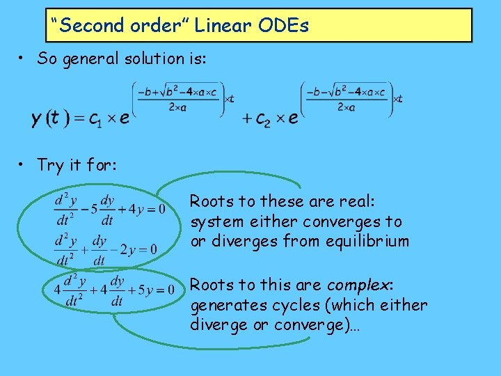
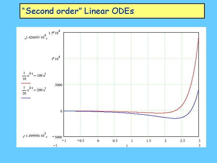
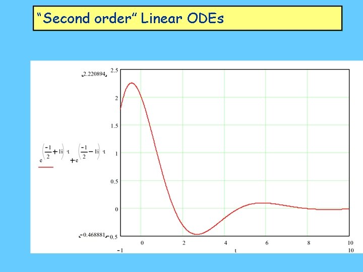
“Second order” Linear ODEs • So general solution is: • Try it for: Roots to these are real: system either converges to or diverges from equilibrium Roots to this are complex: generates cycles (which either diverge or converge)…

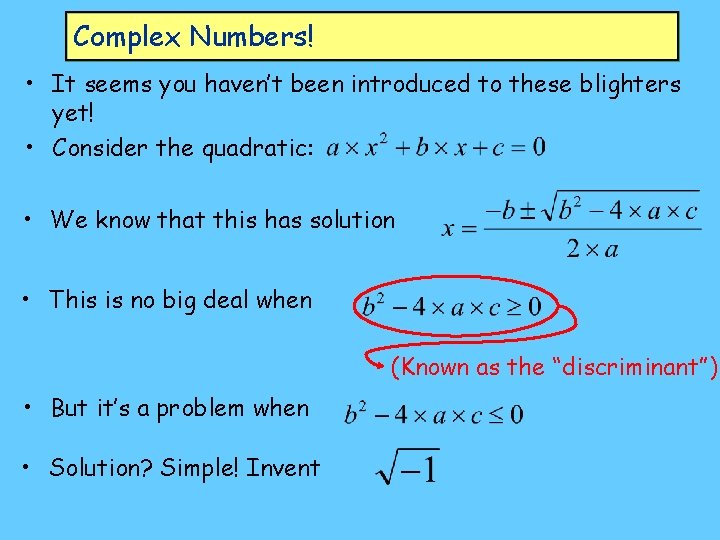
Complex Numbers! • It seems you haven’t been introduced to these blighters yet! • Consider the quadratic: • We know that this has solution • This is no big deal when (Known as the “discriminant”) • But it’s a problem when • Solution? Simple! Invent

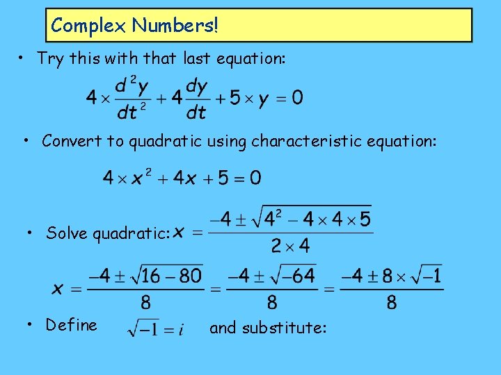
Complex Numbers! • Try this with that last equation: • Convert to quadratic using characteristic equation: • Solve quadratic: • Define and substitute:

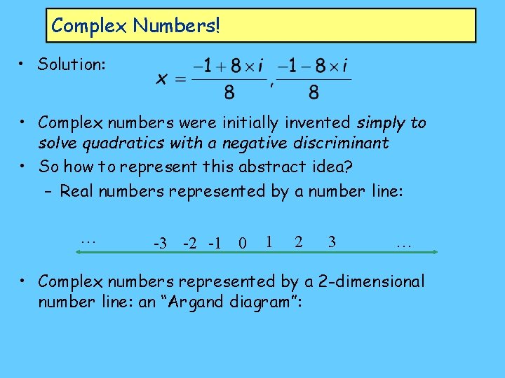
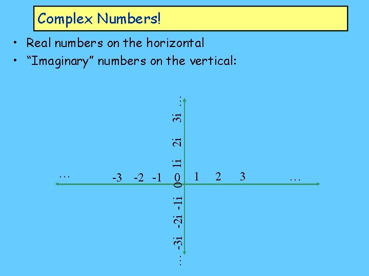
Complex Numbers! • Solution: • Complex numbers were initially invented simply to solve quadratics with a negative discriminant • So how to represent this abstract idea? – Real numbers represented by a number line: … -3 -2 -1 0 1 2 3 … • Complex numbers represented by a 2 -dimensional number line: an “Argand diagram”:

Complex Numbers! -3 -2 -1 0 … -3 i -2 i -1 i 0 … 1 i 2 i 3 i … • Real numbers on the horizontal • “Imaginary” numbers on the vertical: 1 2 3 …

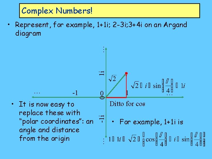
Complex Numbers! 1 i … • Represent, for example, 1+1 i; 2 -3 i; 3+4 i on an Argand diagram 0 • It is now easy to replace these with “polar coordinates”: an angle and distance from the origin 0 1 … Ditto for cos -1 i -1 … … • For example, 1+1 i is

Complex solutions to ODEs • For a complex number to be zero, both its real and imaginary parts must be zero • The real components of the real (cos(bt)) and imaginary (isin(bt)) parts of complex root to a characteristic equation are linearly independent • These two parts alone thus provide the two linearly independent solutions to a second order ODE: the imaginary i can be dropped. – A bit more explanation:

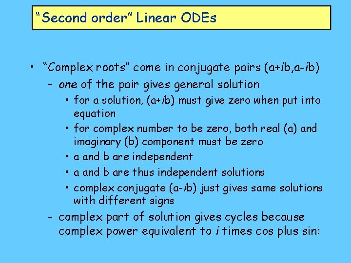
“Second order” Linear ODEs • “Complex roots” come in conjugate pairs (a+ib, a-ib) – one of the pair gives general solution • for a solution, (a+ib) must give zero when put into equation • for complex number to be zero, both real (a) and imaginary (b) component must be zero • a and b are independent • a and b are thus independent solutions • complex conjugate (a-ib) just gives same solutions with different signs – complex part of solution gives cycles because complex power equivalent to i times cos plus sin:

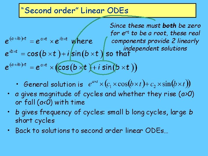
“Second order” Linear ODEs Since these must both be zero for ert to be a root, these real components provide 2 linearly independent solutions • General solution is • a gives magnitude of cycles and whether they rise (a>0) or fall (a<0) with time • b gives frequency of cycles: small b long cycles, large b short cycles • Back to solutions to second order linear ODEs…

“Second order” Linear ODEs

“Second order” Linear ODEs

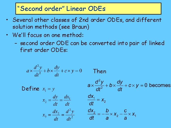
“Second order” Linear ODEs • Several other classes of 2 nd order ODEs, and different solution methods (see Braun) • We’ll focus on one method: – second order ODE can be converted into pair of linked first order ODEs: Then Define

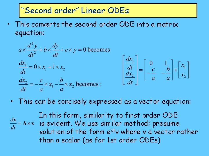
“Second order” Linear ODEs • This converts the second order ODE into a matrix equation: • This can be concisely expressed as a vector equation: In this form, similarity to first order ODE is evident. We use similar method: presume solution of the form eltv where v a vector rather than a scalar (as for 1 st order ODEs)

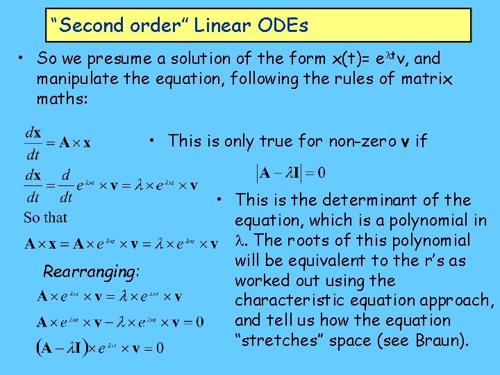
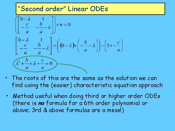
“Second order” Linear ODEs • So we presume a solution of the form x(t)= eltv, and manipulate the equation, following the rules of matrix maths: • This is only true for non-zero v if Rearranging: • This is the determinant of the equation, which is a polynomial in l. The roots of this polynomial will be equivalent to the r’s as worked out using the characteristic equation approach, and tell us how the equation “stretches” space (see Braun).

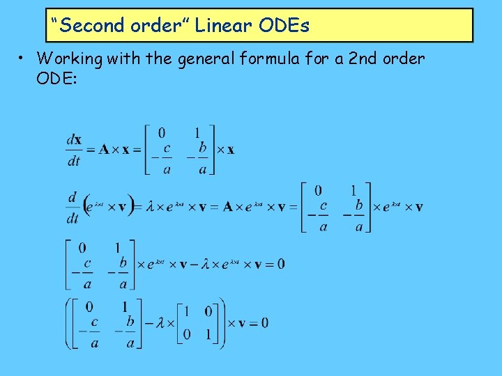
“Second order” Linear ODEs • Working with the general formula for a 2 nd order ODE:

“Second order” Linear ODEs • The roots of this are the same as the solution we can find using the (easier) characteristic equation approach • Method useful when doing third or higher order ODEs (there is no formula for a 6 th order polynomial or above; 3 rd & above formulas are a mess!)

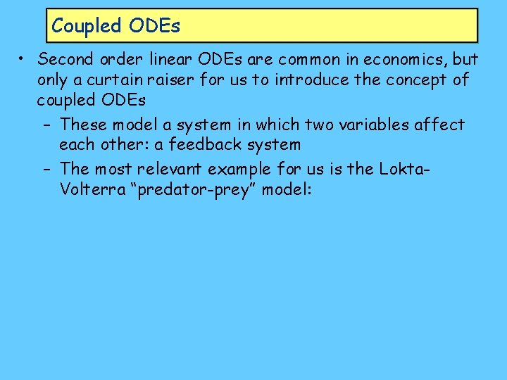
Coupled ODEs • Second order linear ODEs are common in economics, but only a curtain raiser for us to introduce the concept of coupled ODEs – These model a system in which two variables affect each other: a feedback system – The most relevant example for us is the Lokta. Volterra “predator-prey” model:

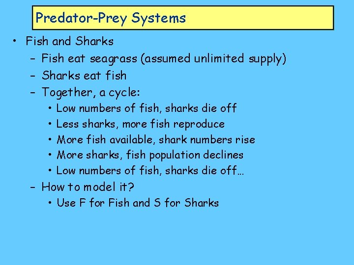
Predator-Prey Systems • Fish and Sharks – Fish eat seagrass (assumed unlimited supply) – Sharks eat fish – Together, a cycle: • • • Low numbers of fish, sharks die off Less sharks, more fish reproduce More fish available, shark numbers rise More sharks, fish population declines Low numbers of fish, sharks die off… – How to model it? • Use F for Fish and S for Sharks

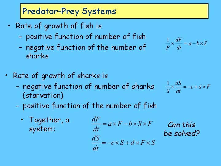
Predator-Prey Systems • Rate of growth of fish is – positive function of number of fish – negative function of the number of sharks • Rate of growth of sharks is – negative function of number of sharks (starvation) – positive function of the number of fish • Together, a system: Can this be solved?

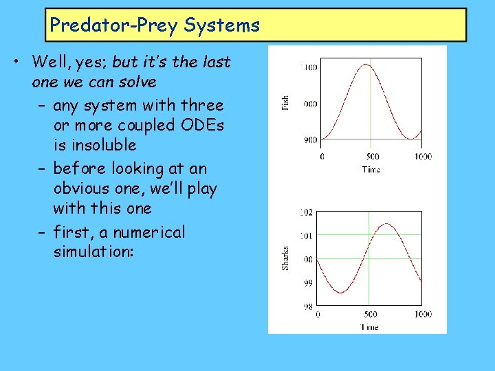
Predator-Prey Systems • Well, yes; but it’s the last one we can solve – any system with three or more coupled ODEs is insoluble – before looking at an obvious one, we’ll play with this one – first, a numerical simulation:

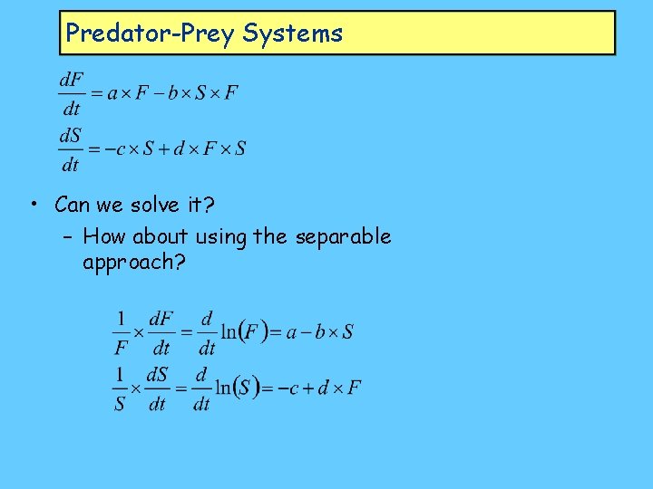
Predator-Prey Systems • Can we solve it? – How about using the separable approach?

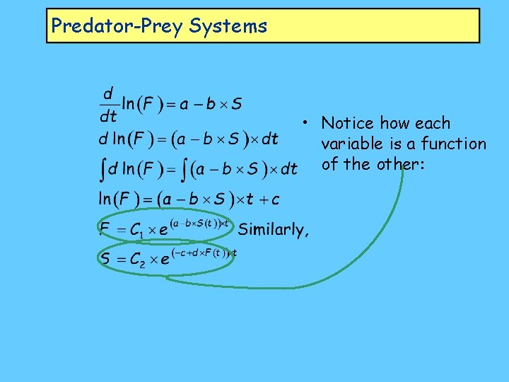
Predator-Prey Systems • Notice how each variable is a function of the other:

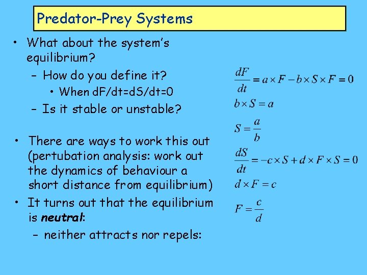
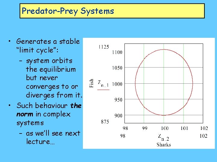
Predator-Prey Systems • What about the system’s equilibrium? – How do you define it? • When d. F/dt=d. S/dt=0 – Is it stable or unstable? • There are ways to work this out (pertubation analysis: work out the dynamics of behaviour a short distance from equilibrium) • It turns out that the equilibrium is neutral: – neither attracts nor repels:

Predator-Prey Systems • Generates a stable “limit cycle”: – system orbits the equilibrium but never converges to or diverges from it. • Such behaviour the norm in complex systems – as we’ll see next lecture…