Advanced Algorithm Design and Analysis Lecture 1 SW

Advanced Algorithm Design and Analysis (Lecture 1) SW 5 fall 2004 Simonas Šaltenis E 1 -215 b simas@cs. aau. dk AALG, lecture 1, © Simonas Šaltenis, 2004

Overview n n n Why do we need this course? Goals of the course Mode of work Prerequisites, textbook The first lecture – external data structures AALG, lecture 1, © Simonas Šaltenis, 2004 2

External Mem. Data Structures n Goals of the lecture: n n n to understand the external memory model and the principles of analysis of algorithms and data structures in this model; to understand why main-memory algorithms are not efficient in external memory; to understand the algorithms of B-tree and its variants and to be able to analyze them. AALG, lecture 1, © Simonas Šaltenis, 2004 3

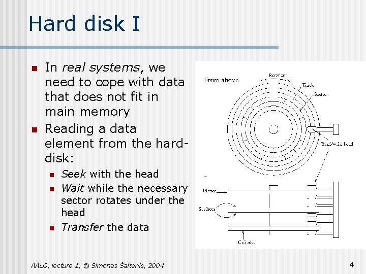
Hard disk I n n In real systems, we need to cope with data that does not fit in main memory Reading a data element from the harddisk: n n n Seek with the head Wait while the necessary sector rotates under the head Transfer the data AALG, lecture 1, © Simonas Šaltenis, 2004 4

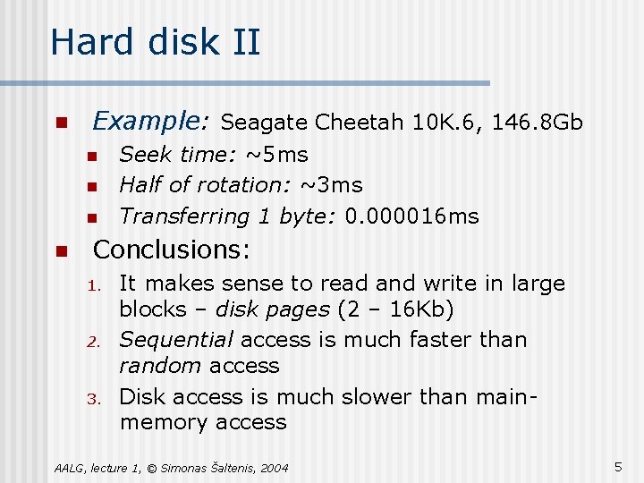
Hard disk II n Example: Seagate Cheetah 10 K. 6, 146. 8 Gb n n Seek time: ~5 ms Half of rotation: ~3 ms Transferring 1 byte: 0. 000016 ms Conclusions: 1. 2. 3. It makes sense to read and write in large blocks – disk pages (2 – 16 Kb) Sequential access is much faster than random access Disk access is much slower than mainmemory access AALG, lecture 1, © Simonas Šaltenis, 2004 5

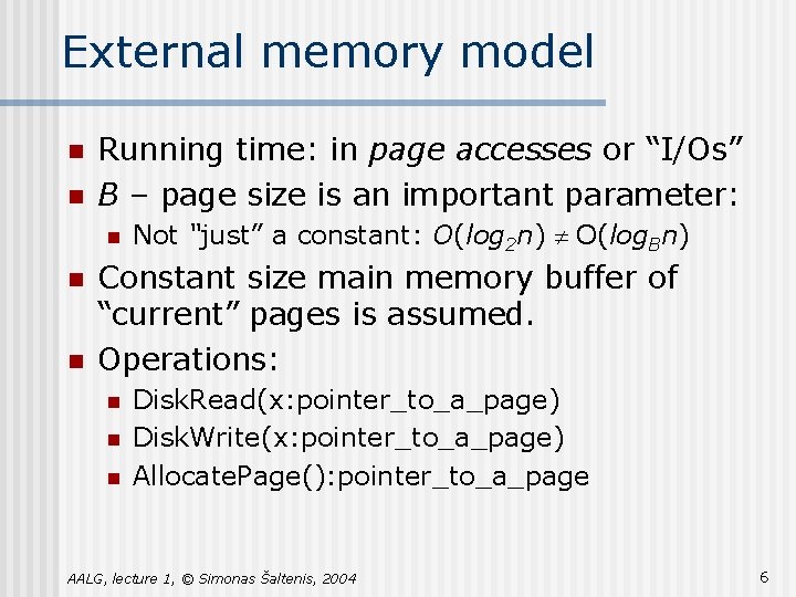
External memory model n n Running time: in page accesses or “I/Os” B – page size is an important parameter: n n n Not “just” a constant: O(log 2 n) ¹ O(log. Bn) Constant size main memory buffer of “current” pages is assumed. Operations: n n n Disk. Read(x: pointer_to_a_page) Disk. Write(x: pointer_to_a_page) Allocate. Page(): pointer_to_a_page AALG, lecture 1, © Simonas Šaltenis, 2004 6

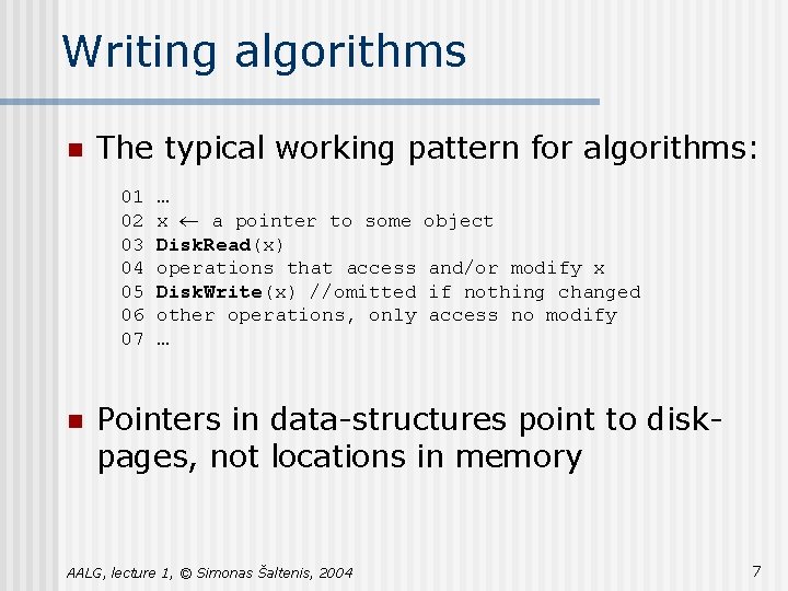
Writing algorithms n The typical working pattern for algorithms: 01 … 02 x ¬ a pointer to some object 03 Disk. Read(x) 04 operations that access and/or modify x 05 Disk. Write(x) //omitted if nothing changed 06 other operations, only access no modify 07 … n Pointers in data-structures point to diskpages, not locations in memory AALG, lecture 1, © Simonas Šaltenis, 2004 7

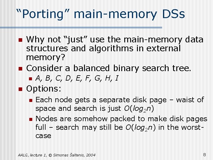
“Porting” main-memory DSs n n Why not “just” use the main-memory data structures and algorithms in external memory? Consider a balanced binary search tree. n n A, B, C, D, E, F, G, H, I Options: n n Each node gets a separate disk page – waist of space and search is just O(log 2 n) Nodes are somehow packed to make disk pages full – search may still be O(log 2 n) in the worstcase AALG, lecture 1, © Simonas Šaltenis, 2004 8

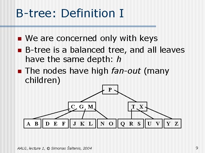
B-tree: Definition I n n n We are concerned only with keys B-tree is a balanced tree, and all leaves have the same depth: h The nodes have high fan-out (many children) P C G M A B D E F J K L AALG, lecture 1, © Simonas Šaltenis, 2004 T X N O Q R S U V Y Z 9

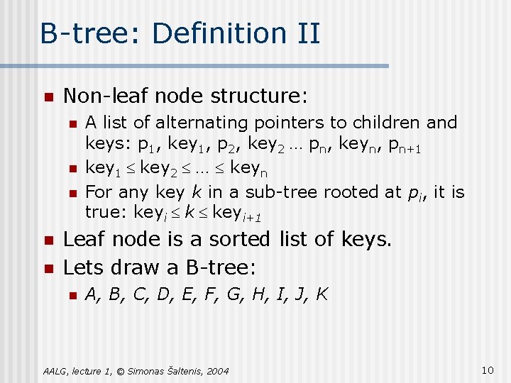
B-tree: Definition II n Non-leaf node structure: n n n A list of alternating pointers to children and keys: p 1, key 1, p 2, key 2 … pn, keyn, pn+1 key 1 £ key 2 £ … £ keyn For any key k in a sub-tree rooted at pi, it is true: keyi £ keyi+1 Leaf node is a sorted list of keys. Lets draw a B-tree: n A, B, C, D, E, F, G, H, I, J, K AALG, lecture 1, © Simonas Šaltenis, 2004 10

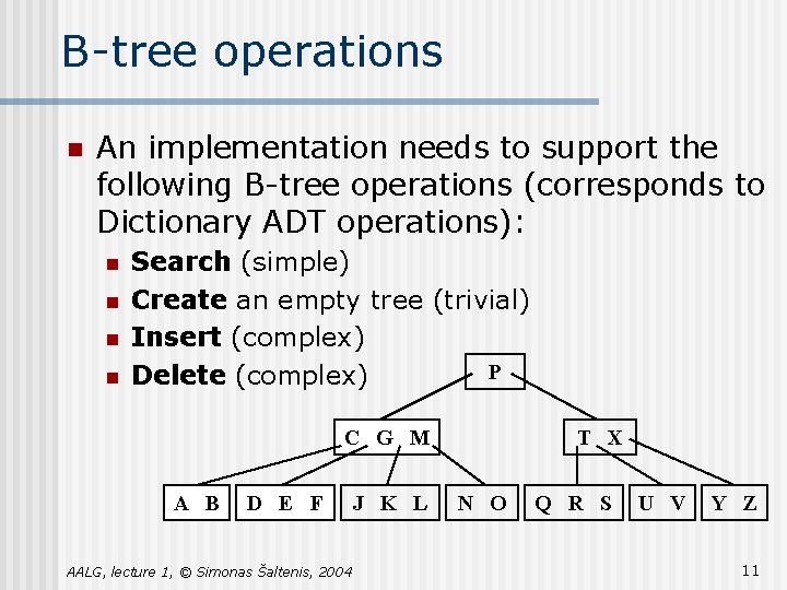
B-tree operations n An implementation needs to support the following B-tree operations (corresponds to Dictionary ADT operations): n n Search (simple) Create an empty tree (trivial) Insert (complex) P Delete (complex) C G M A B D E F AALG, lecture 1, © Simonas Šaltenis, 2004 J K L T X N O Q R S U V Y Z 11

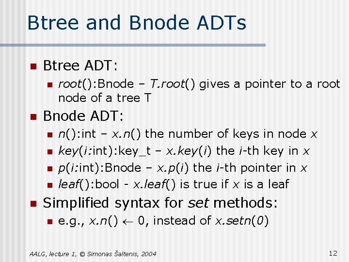
Btree and Bnode ADTs n Btree ADT: n n Bnode ADT: n n n root(): Bnode – T. root() gives a pointer to a root node of a tree T n(): int – x. n() the number of keys in node x key(i: int): key_t – x. key(i) the i-th key in x p(i: int): Bnode – x. p(i) the i-th pointer in x leaf(): bool - x. leaf() is true if x is a leaf Simplified syntax for set methods: n e. g. , x. n() ¬ 0, instead of x. setn(0) AALG, lecture 1, © Simonas Šaltenis, 2004 12

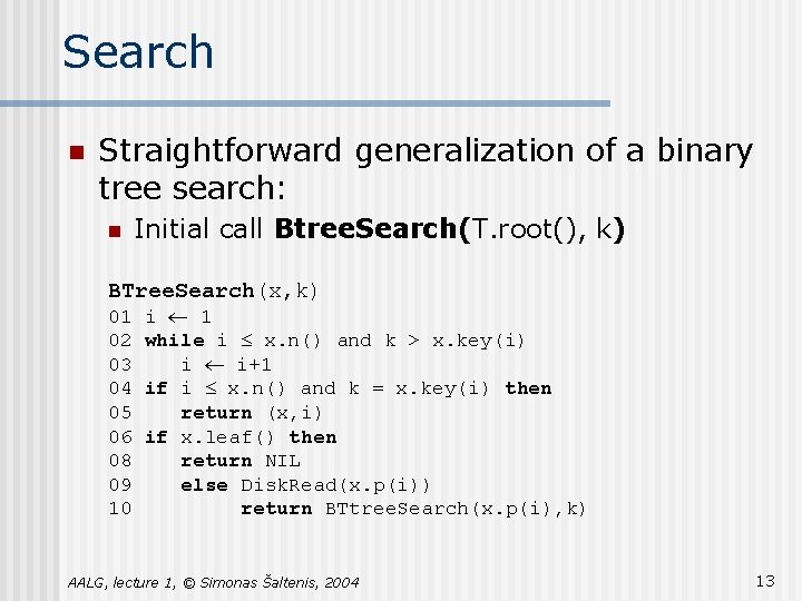
Search n Straightforward generalization of a binary tree search: n Initial call Btree. Search(T. root(), k) BTree. Search(x, k) 01 i ¬ 1 02 while i £ x. n() and k > x. key(i) 03 i ¬ i+1 04 if i £ x. n() and k = x. key(i) then 05 return (x, i) 06 if x. leaf() then 08 return NIL 09 else Disk. Read(x. p(i)) 10 return BTtree. Search(x. p(i), k) AALG, lecture 1, © Simonas Šaltenis, 2004 13

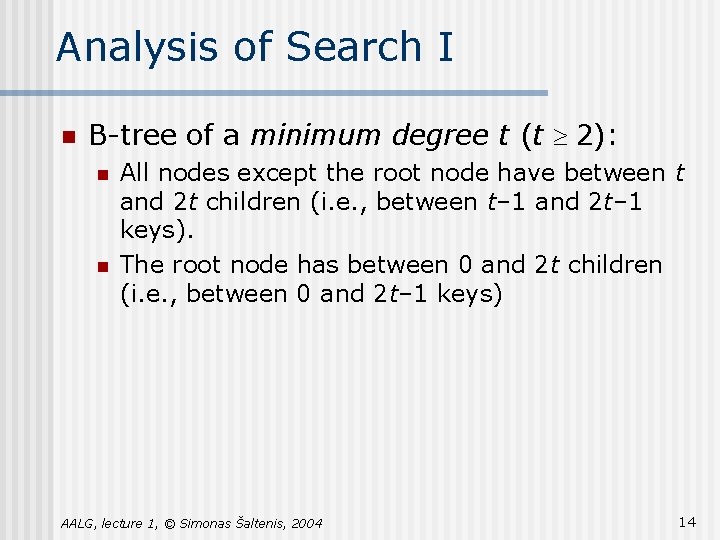
Analysis of Search I n B-tree of a minimum degree t (t ³ 2): n n All nodes except the root node have between t and 2 t children (i. e. , between t– 1 and 2 t– 1 keys). The root node has between 0 and 2 t children (i. e. , between 0 and 2 t– 1 keys) AALG, lecture 1, © Simonas Šaltenis, 2004 14

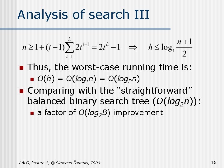
Analysis of Search II n For B-tree containing n ³ 1 keys and minimum degree t ³ 2, the following restriction on the height h holds: n Why? The highest tree: depth 1 t-1 t t-1 #of nodes 0 1 1 2 2 2 t t t-1 … t-1 AALG, lecture 1, © Simonas Šaltenis, 2004 t-1 … t-1 15

Analysis of search III n Thus, the worst-case running time is: n n O(h) = O(logtn) = O(log. Bn) Comparing with the “straightforward” balanced binary search tree (O(log 2 n)): n a factor of O(log 2 B) improvement AALG, lecture 1, © Simonas Šaltenis, 2004 16

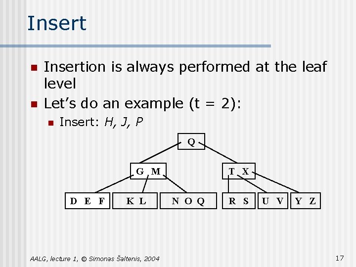
Insert n n Insertion is always performed at the leaf level Let’s do an example (t = 2): n Insert: H, J, P Q G M D E F K L AALG, lecture 1, © Simonas Šaltenis, 2004 T X N O Q R S U V Y Z 17

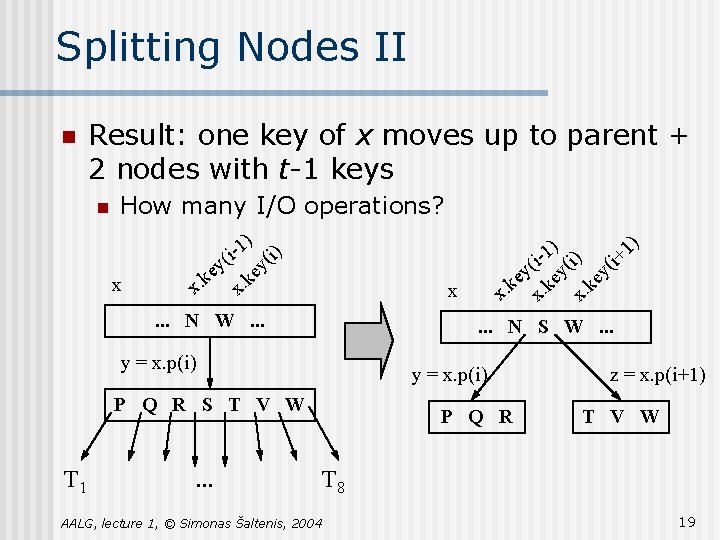
Splitting Nodes n n Nodes fill up and reach their maximum capacity 2 t – 1 Before we can insert a new key, we have to “make room, ” i. e. , split a node AALG, lecture 1, © Simonas Šaltenis, 2004 18

Splitting Nodes II Result: one key of x moves up to parent + 2 nodes with t-1 keys ) ) . . . N W. . . y = x. p(i) P Q R S T V W . . . ke . . . N S W. . . y = x. p(i) T 1 k x. x y( i) ke x x. x ey k. i-1 ( ey x. 1 (i- y( i+ 1) How many I/O operations? ke n x. n P Q R z = x. p(i+1) T V W T 8 AALG, lecture 1, © Simonas Šaltenis, 2004 19

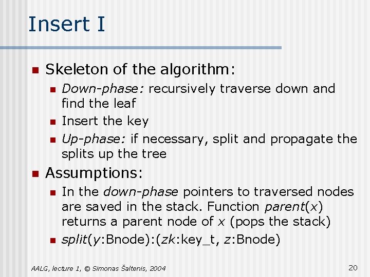
Insert I n Skeleton of the algorithm: n n Down-phase: recursively traverse down and find the leaf Insert the key Up-phase: if necessary, split and propagate the splits up the tree Assumptions: n n In the down-phase pointers to traversed nodes are saved in the stack. Function parent(x) returns a parent node of x (pops the stack) split(y: Bnode): (zk: key_t, z: Bnode) AALG, lecture 1, © Simonas Šaltenis, 2004 20

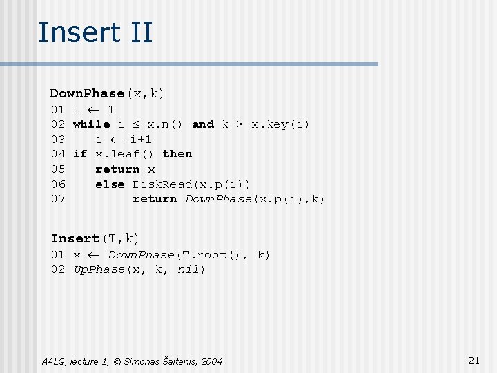
Insert II Down. Phase(x, k) 01 i ¬ 1 02 while i £ x. n() and k > x. key(i) 03 i ¬ i+1 04 if x. leaf() then 05 return x 06 else Disk. Read(x. p(i)) 07 return Down. Phase(x. p(i), k) Insert(T, k) 01 x ¬ Down. Phase(T. root(), k) 02 Up. Phase(x, k, nil) AALG, lecture 1, © Simonas Šaltenis, 2004 21

Insert III Up. Phase(x, k, p) 01 if x. n() = 2 t-1 then 02 (zk, z) ¬ split(x) 03 if k £ zk then Insert. Into. Node(x, k, p) 04 else Insert. Into. Node(z, k, p) 05 if parent(x)=nil then (Create new root) 06 else Up. Phase(parent(x), zk, z) 07 else Insert. Into. Node(x, k, p) Inserts the hey k and the following pointer p (if not nil) into the sorted order of keys of x, so that all the keys before k are smaller or equal to k and all the keys after k are greater than k AALG, lecture 1, © Simonas Šaltenis, 2004 22

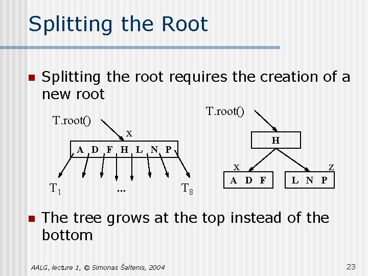
Splitting the Root n Splitting the root requires the creation of a new root T. root() x H A D F H L N P x T 1 n . . . T 8 A D F z L N P The tree grows at the top instead of the bottom AALG, lecture 1, © Simonas Šaltenis, 2004 23

One/Two Phase Algorithms n n n Running time: O(h) = O(log. Bn) Insert could be done in one traversal down the tree (by splitting all full nodes that we meet, “just in case”) Disadvantage of the two-phase algorithm: n Buffer of O(h) pages is required AALG, lecture 1, © Simonas Šaltenis, 2004 24

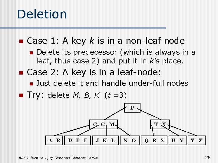
Deletion n Case 1: A key k is in a non-leaf node n n Case 2: A key is in a leaf-node: n n Delete its predecessor (which is always in a leaf, thus case 2) and put it in k’s place. Just delete it and handle under-full nodes Try: delete M, B, K (t =3) P C G M A B D E F J K L AALG, lecture 1, © Simonas Šaltenis, 2004 T X N O Q R S U V Y Z 25

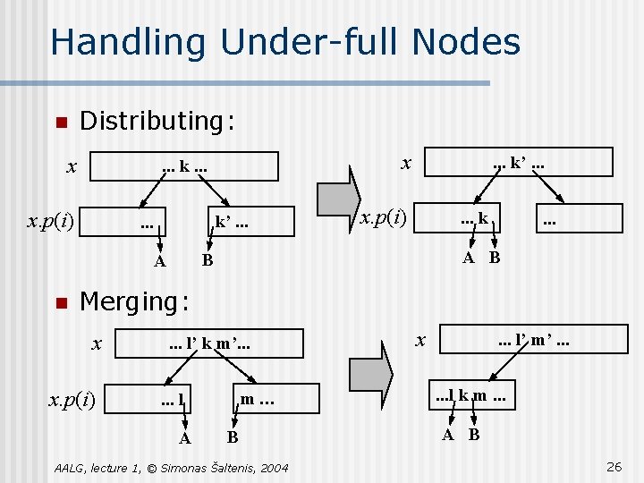
Handling Under-full Nodes n Distributing: x x. p(i) k’. . . x. p(i) . . . k . . . A B B A n x . . . k. . . Merging: x x. p(i) . . . l’ k m’. . . m… . . . l A B AALG, lecture 1, © Simonas Šaltenis, 2004 x . . . l’ m’. . . l k m. . . A B 26

Sequential access n Other useful ADT operator: successor n n For example, range queries: find all accounts with the amount in the range [100 K – 200 K]. How do you do that in B-trees? AALG, lecture 1, © Simonas Šaltenis, 2004 27

B+-trees n B+-trees is a variant of B-trees: n All data keys are in leaf nodes • The split does not move the middle key to the parent, but copies it to the parent! n n Leaf-nodes are connected into a (doubly) linked list How the range query is performed? • Compare with the B-tree AALG, lecture 1, © Simonas Šaltenis, 2004 28