Lecture 4 Nonlinear price discrimination Nonlinear prices In

Lecture 4 Non-linear price discrimination

Non-linear prices • In chapter 5, we looked at price discrimination schemes where we charged consumers a constant linear price per unit. • In practice, we often observe pricing schemes that are nonlinear (bulk discounts, for example). While often these represent decreasing average costs at higher quantities (eg; buying 2000 cans of coke rather than a single can), they are also often the result of a price discrimination policy. • Why nonlinear prices? Either because these allow the firm to increase profits even more than a linear price would (1 st degree PD) or because the firm is unable to separate consumer types (2 nd degree PD).

First degree PD (“personalized pricing”) • • First degree price discrimination is when the monopolist is able to charge the maximum price each consumer is willing to pay for each unit of product sold. Suppose you are selling off a new subdivision of 6 identical houses. Suppose that there are two buyers willing to pay $400 k, one buyer willing to pay $380 k, 1 buyer willing to pay $360 k, 2 buyers willing to pay $350 k and three buyers willing to pay $330 k. To sell all 6 houses with a linear price, we would only be able to charge $350 k for total revenue $2. 1 million. But with a nonlinear price, we could charge exactly the willingness to pay of the top 6 buyers, yielding revenue $2. 24 million. Even if consumers had different willingness to pay for different units (eg they are willing to pay $30 k for one car but only $10 k for a second), a monopolist can charge the marginal willingness to pay for each unit. Since first degree PD redirects surplus from consumers to producers, it provides incentives for monopolists to produce more. Under first-degree PD, the monopolist chooses the same socially efficient quantity that would be generated under perfect competition. By capturing all consumer surplus, the monopolist maximizing producer surplus is doing the same as a social planner maximizing total surplus.

Two-part tariffs • • In practice, pure first degree price discrimination is very rarely seen in practice, if ever. The monopolist has to know the exact willingness to pay of consumers, and to be able to distinguish all consumer types, and prevent arbitrage. A more commonly observed technique which achieves the same effect is known as “two-part pricing” or “two-part tariffs”. A two-part tariff consists of a marginal cost per unit, and a flat “fee” that must be paid for the right to purchase goods at that marginal cost. The marginal fee is the same for all users, which prevents arbitrage. Examples: Bar cover charges. Private clubs. Costco Amusement parks. Professional services (lawyers, lobbyists, etc. )

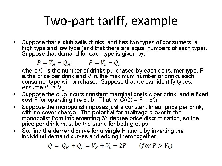
Two-part tariff, example • • Suppose that a club sells drinks, and has two types of consumers, a high type and low type (and that there are equal numbers of each type). Suppose that demand for each type is given by: where Qi is the number of drinks purchased by each consumer type, P is the price per drink and Vi is the maximum number of drinks each consumer type will purchase. Suppose that we can identify types. Assume VH > VL. Suppose the club incurs constant marginal costs c per drink, and a fixed cost F for operating the club. That is, C(Q) = F + c. Q. Suppose the monopolist imposes just a constant linear price per drink, with no cover charge. The potential for arbitrage prevents the monopolist from implementing 3 rd degree price discrimination, so the price per drink must be the same for both groups. So, find the demand curve for a single H and L by inverting the individual demand curves and adding them together.

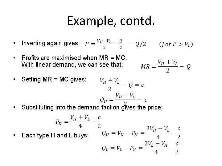
Example, contd. • Inverting again gives: • Profits are maximised when MR = MC. With linear demand, we can see that: • Setting MR = MC gives: • Substituting into the demand faction gives the price: • Each type H and L buys:

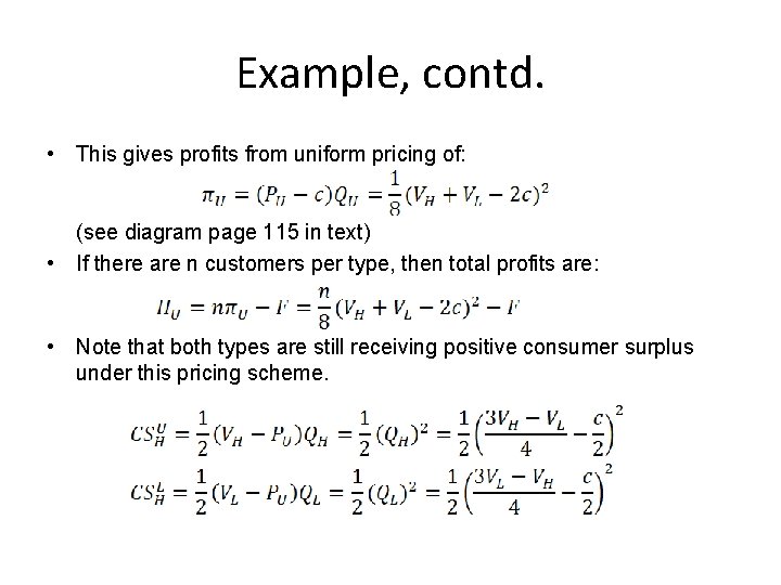
Example, contd. • This gives profits from uniform pricing of: (see diagram page 115 in text) • If there are n customers per type, then total profits are: • Note that both types are still receiving positive consumer surplus under this pricing scheme.

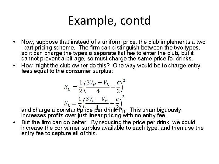
Example, contd • • • Now, suppose that instead of a uniform price, the club implements a two -part pricing scheme. The firm can distinguish between the two types, so it can charge the types a separate flat fee to enter the club, but it cannot prevent arbitrage, so must charge the same price for drinks. How might the club owner do this? One way would be to charge entry fees equal to the consumer surplus: and charge a constant price per drink PU. This unambiguously increases profits over just linear pricing with no entry fee. But the firm can do better. By reducing the price per drink, we could increase the consumer surplus available to each type, and then use the entry fee to capture all of this.

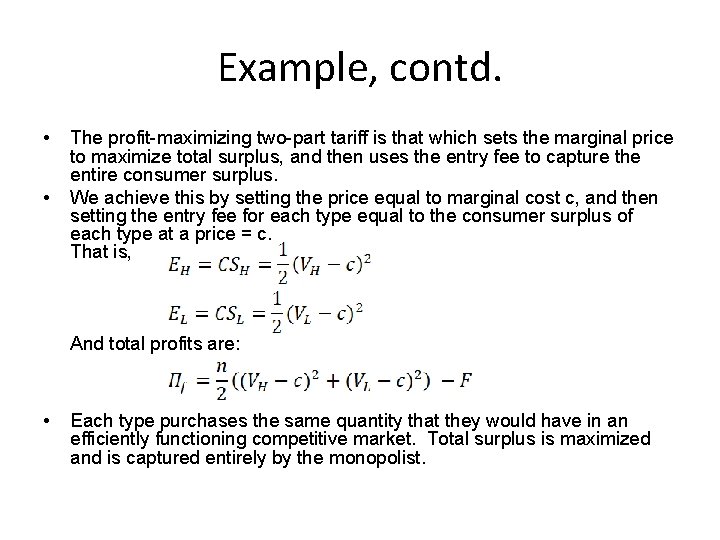
Example, contd. • • The profit-maximizing two-part tariff is that which sets the marginal price to maximize total surplus, and then uses the entry fee to capture the entire consumer surplus. We achieve this by setting the price equal to marginal cost c, and then setting the entry fee for each type equal to the consumer surplus of each type at a price = c. That is, And total profits are: • Each type purchases the same quantity that they would have in an efficiently functioning competitive market. Total surplus is maximized and is captured entirely by the monopolist.

Block pricing • “Block pricing” is another form of first degree PD that can achieve the same result as a 2 -part tariff. Rather than setting a marginal tariff per unit of output for all groups and charging a fixed cost that varies by groups, we can instead sell “bundles” to different types of consumer. These bundles are contracts of the form “Entry and X “free” drinks for Y dollars”. • Optimal pricing under this rule is simple. 1. Set the quantity offered to each consumer type equal to the amount that consumer would buy under competitive pricing (P=MC). 2. Set a fixed charge for each consumer type at the total willingness to pay for the quantity identified above. • So we are duplicating the result of the two-part tariff scheme, but doing it by only charging each customer one single charge rather than multiple times (entry plus price per drink).

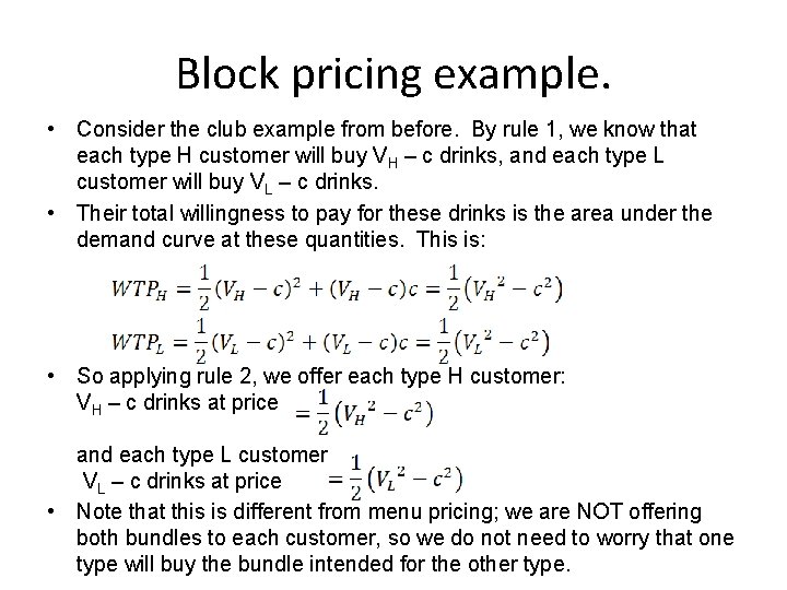
Block pricing example. • Consider the club example from before. By rule 1, we know that each type H customer will buy VH – c drinks, and each type L customer will buy VL – c drinks. • Their total willingness to pay for these drinks is the area under the demand curve at these quantities. This is: • So applying rule 2, we offer each type H customer: VH – c drinks at price and each type L customer VL – c drinks at price • Note that this is different from menu pricing; we are NOT offering both bundles to each customer, so we do not need to worry that one type will buy the bundle intended for the other type.

Example, contd • Profit from a customer of type i is the WTPi minus the cost of the drinks c(Vi – c), or (Vi-c)2/2, exactly as in the two-part tariff system. • Note that both the two-part tariff and the block-pricing schemes result in the club owner serving both types of quantity the same quantity at the same total price. • The average price paid by each customer type per unit is different; the high type ends up paying a higher price. • These average prices are the same as would be levied if the club were to apply a third-degree price discrimination (check this yourself). • But; the profit outcome is different. The club owner yields higher profits (and sells higher quantity) under first degree price discrimination than under third degree price discrimination. The club owner is appropriating all consumer surplus, which they were unable to do with third degree price discrimination.

Second degree PD: Menu pricing • Recall that for first or second degree PD to be possible, we had to be able to distinguish between types, either to charge them different marginal prices (3 rd degree), different entry charges (two-part tariff) or offer them different bundles (block pricing). The monopolist could prevent a consumer from purchasing at a price or bundle not intended for their type. What if this is not possible? • If we could not identify the type of a particular consumer (or could not price based on this, because of practicalities or antidiscrimination laws), then these methods would fail. • Second degree PD offers a way to discriminate even if we cannot observe the type of a particular consumer (though we must still know the properties of each type in general). We design a pricing scheme that will induce customers into voluntarily revealing their own type. We do this by offering all customers a menu of price/quantity bundles, and letting each customer choose the bundle that suits them best.

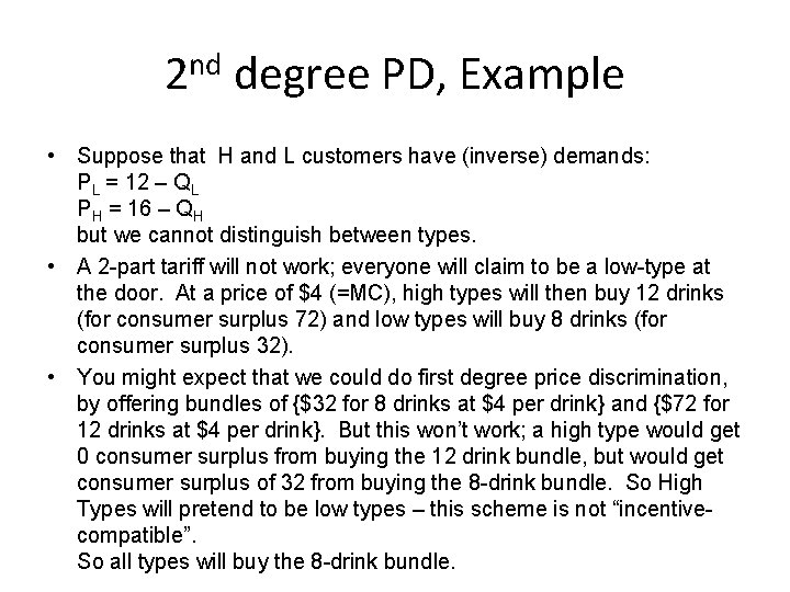
2 nd degree PD, Example • Suppose that H and L customers have (inverse) demands: PL = 12 – QL PH = 16 – QH but we cannot distinguish between types. • A 2 -part tariff will not work; everyone will claim to be a low-type at the door. At a price of $4 (=MC), high types will then buy 12 drinks (for consumer surplus 72) and low types will buy 8 drinks (for consumer surplus 32). • You might expect that we could do first degree price discrimination, by offering bundles of {$32 for 8 drinks at $4 per drink} and {$72 for 12 drinks at $4 per drink}. But this won’t work; a high type would get 0 consumer surplus from buying the 12 drink bundle, but would get consumer surplus of 32 from buying the 8 -drink bundle. So High Types will pretend to be low types – this scheme is not “incentivecompatible”. So all types will buy the 8 -drink bundle.

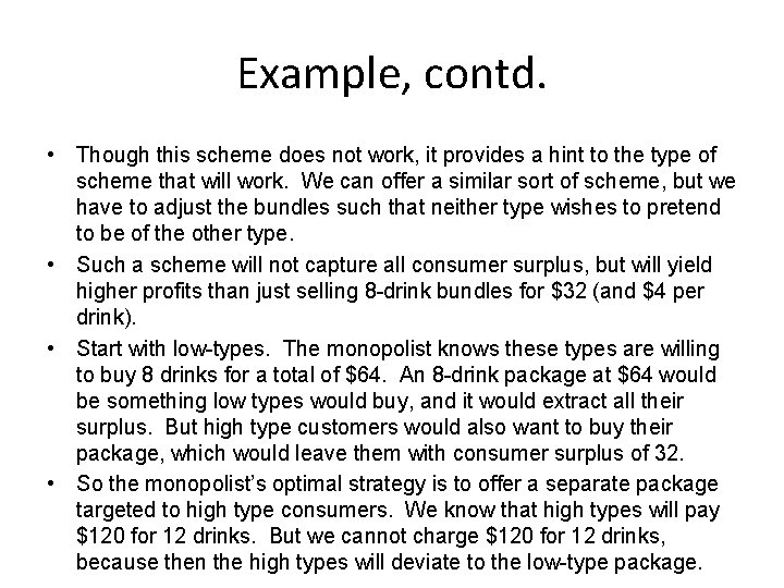
Example, contd. • Though this scheme does not work, it provides a hint to the type of scheme that will work. We can offer a similar sort of scheme, but we have to adjust the bundles such that neither type wishes to pretend to be of the other type. • Such a scheme will not capture all consumer surplus, but will yield higher profits than just selling 8 -drink bundles for $32 (and $4 per drink). • Start with low-types. The monopolist knows these types are willing to buy 8 drinks for a total of $64. An 8 -drink package at $64 would be something low types would buy, and it would extract all their surplus. But high type customers would also want to buy their package, which would leave them with consumer surplus of 32. • So the monopolist’s optimal strategy is to offer a separate package targeted to high type consumers. We know that high types will pay $120 for 12 drinks. But we cannot charge $120 for 12 drinks, because then the high types will deviate to the low-type package.

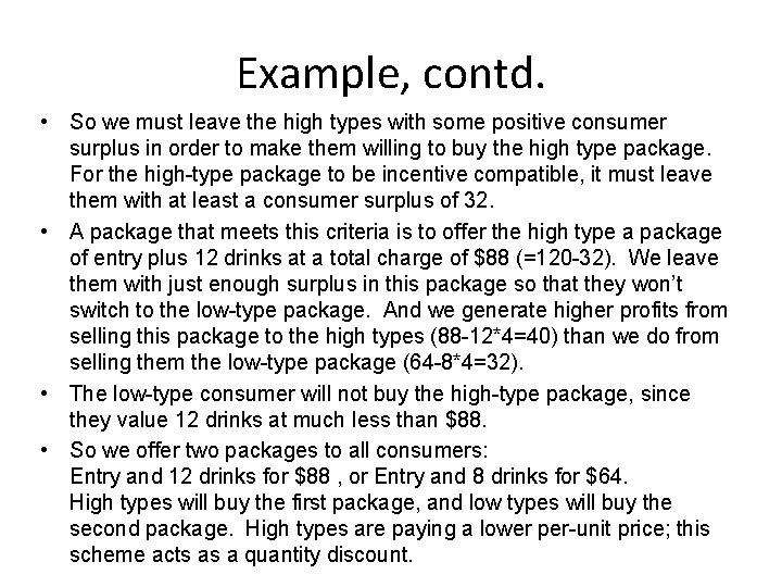
Example, contd. • So we must leave the high types with some positive consumer surplus in order to make them willing to buy the high type package. For the high-type package to be incentive compatible, it must leave them with at least a consumer surplus of 32. • A package that meets this criteria is to offer the high type a package of entry plus 12 drinks at a total charge of $88 (=120 -32). We leave them with just enough surplus in this package so that they won’t switch to the low-type package. And we generate higher profits from selling this package to the high types (88 -12*4=40) than we do from selling them the low-type package (64 -8*4=32). • The low-type consumer will not buy the high-type package, since they value 12 drinks at much less than $88. • So we offer two packages to all consumers: Entry and 12 drinks for $88 , or Entry and 8 drinks for $64. High types will buy the first package, and low types will buy the second package. High types are paying a lower per-unit price; this scheme acts as a quantity discount.

2 nd degree PD • Quantity discounts such as this are common. It is cheaper to buy a large bag of rice (per unit) than a small one. Wine sold by the glass is more expensive than buying an entire bottle. A 24 -back of Coke is cheaper than buying 24 individual cans. A season ticket costs less than buying tickets for every event. Some of this difference can be explained by cost differences, but the rest is a form of 2 nd degree price discrimination, where the firm induces you to reveal your type.

Example, contd • But even this package is not optimal. Suppose now that we were to offer a lower number of drinks in the low-type package; say we reduce this to 7 drinks. The low-demand customer is willing to pay $59. 50 for this package. By doing this, we reduce the profit gained from low-type customers (to $31. 50). • But by lowering the value of the low-type bundle, we have relaxed the incentive compatibility constraint. We can also lower the value of the bundle offered to the high demand customers. Their maximum WTP for 7 drinks is $87. 50, so buying this package leaves them with only a surplus of $28. As a result, the club owner can increase the price of the 12 -drink package without violating the incentive compatibility constraint. • We can increase the price of the high-type package to be 120 – 28 = $92, increasing our profit from this package to $44. So we are losing $0. 50 per low type to gain $4 per high type. • The optimal package will depend on the relative numbers of low and high types.

Optimal 2 nd degree PD. • For the general case of more than two types of customers, the profitmaximizing second-degree pricing scheme will exhibit some key features. If consumer willingness to pay can be unambiguously ranked by type, then any optimal 2 nd degree PD scheme will: 1. Extract the entire consumer surplus of the lowest type served, but leave some consumer surplus for all other types (incentive to induce them to reveal their type). 2. Contain a quantity that is less than the socially optimal quantity for all consumer types other than the highest type. 3. Exhibit quantity discounting. • 2 nd degree PD enhances the ability of the monopolist to convert consumer surplus to profit. It does so less effectively than 1 st degree PD, but it is implementable even when consumer types cannot be observed.

Welfare with 1 st and 2 nd degree PD • First, note that price discrimination increases (decreases) the social welfare from selling to consumer group i if it increases (decreases) the quantity sold to that group in equilibrium. • This is not the same as saying that consumer surplus to group i will increase if the quantity sold to that group increases, because the monopolist may be able to capture that consumer surplus with a fixed charge. • It follows immediately that 1 st degree PD always increases social welfare even though it extracts all consumer surplus; with this pricing policy, every consumer group is sold the socially efficient quantity, where P=MC. • With 2 nd degree PD the answer is not so simple. Under this policy, the highest group gets something near to the socially efficient level, but the monopolist restricts the quantity supplied to lower demand groups, and in some cases does not supply these groups at all.

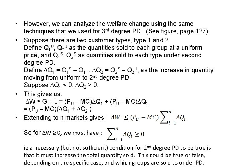
• However, we can analyze the welfare change using the same techniques that we used for 3 rd degree PD. (See figure, page 127). • Suppose there are two customer types, type 1 and 2. Define Q 1 U, Q 2 U as the quantities sold to each group at a uniform price, and Q 1 S, Q 2 S as quantities sold to each type under second degree PD. Define ∆Q 1 = Q 1 S – Q 1 U, ∆Q 2 = Q 2 S – Q 2 U, as the increase in quantity moving from uniform to 2 nd degree PD. Suppose ∆Q 1 < 0, ∆Q 2 > 0. • This gives us: ∆W ≤ G – L = (PU – MC)∆Q 1 + (PU – MC)∆Q 2 = (PU – MC)(∆Q 1 + ∆Q 2 ) • Extending to n markets gives: So for ΔW ≥ 0, we must have : ie a necessary (but not sufficient) condition for 2 nd degree PD to be true is that it must increase the total quantity sold. This could be true or false, depending on the specific case, and which groups are sold to under PD.