Honours Finance Advanced Topics in Finance Nonlinear Analysis

Honours Finance (Advanced Topics in Finance: Nonlinear Analysis) Lecture 4: ODEs continued Coupled ODEs, nonlinearity and the equilibria of nonlinear systems

Recap • Last lecture we considered coupled differential equations, where the level of one variable (a species) depends on itself and another variable • Before considering an economic application of these, I’ll clear up one point concerning complex solutions to second order ODEs. – Remember that • a second order linear ODE can be solved by the characteristic equation method – guess a solution of the form y(t)=ert – substitution converts equation into quadratic in r – complex solution results when b 2 -4 ac<0

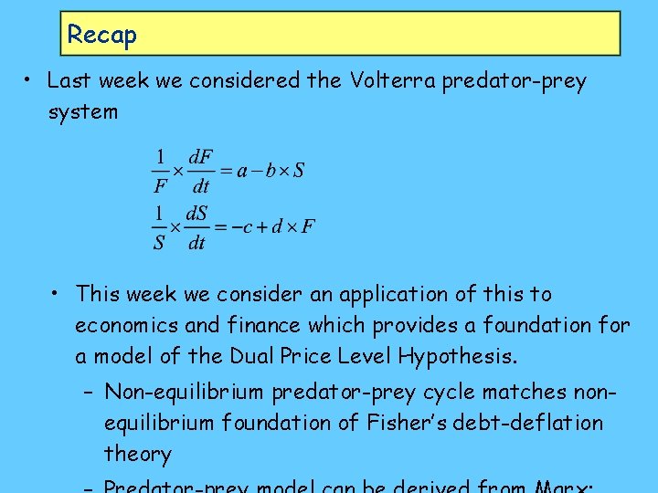
Recap • Last week we considered the Volterra predator-prey system • This week we consider an application of this to economics and finance which provides a foundation for a model of the Dual Price Level Hypothesis. – Non-equilibrium predator-prey cycle matches nonequilibrium foundation of Fisher’s debt-deflation theory

A predator-prey cycle in capitalism • In capitalist, Exchange-Value of work brought to foreground – Exchange-Value of worker=subsistence wage • Use-Value of worker in background: irrelevant to wage – But Use-Value of worker to capitalist purchaser of labour-time=ability to produce commodities for sale • Gap between (objective, quantitative) UV and EV of worker is source of surplus-value (SV) • Analysis presumed labour bought and sold at its value: – cost of production of labour-power • subsistence wage • Is labour actually paid its value in practice?

A predator-prey cycle in capitalism • Many Marxists (especially internationalists like Amin, etc. ) argue labour paid less than its value • But plenty of hints that Marx believed labour paid more than its value: – “the value of the labour-power is equal to the minimum of wages” (1861 I: 46) – “the minimum wage, alias the value of labour-power” (1861 II: 233) – “For the time being, necessary labour supposed as such; i. e. that the worker always obtains only the minimum of wages. ” (1857: 817)

A predator-prey cycle in capitalism • No explanation given by Marx, but can be found in a dialectic of labour: – Worker both a commodity (labour-power) and noncommodity (person) – Capitalism focuses on commodity aspect, pushes noncommodity aspects into background • Pure commodity--paid subsistence wage only • Non-commodity--demands share in surplus • struggle over minimum wage, social wage, etc. – Wage normally exceeds subsistence; subsistence wage a minimum (when commodity aspect dominant and worker power minimal)

A predator-prey cycle in capitalism • “Dialectic of labour” puts into perspective a passage from Marx which is difficult to interpret for “labour is paid less than its value” analysts – “a rise in the price of labor resulting from accumulation of capital implies. . . accumulation slackens in consequence of the rise in the price of labour, because the stimulus of gain is blunted. The rate of accumulation lessens; but with its lessening, the primary cause of that lessening vanishes, i. e. the disproportion between capital and exploitable labour power. The mechanism of the process of capitalist production removes the very obstacles that it temporarily creates. The price of labor falls again to a level corresponding with the needs of the self-expansion of capital, whether the level be below, the same as, or above the one which was normal before the rise of wages took place. . .

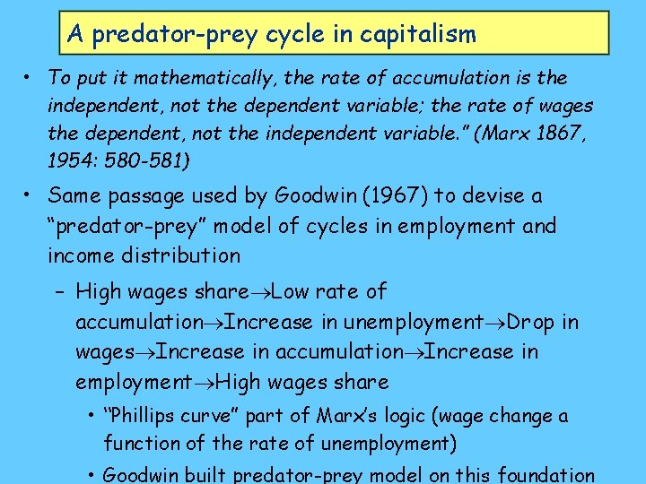
A predator-prey cycle in capitalism • To put it mathematically, the rate of accumulation is the independent, not the dependent variable; the rate of wages the dependent, not the independent variable. ” (Marx 1867, 1954: 580 -581) • Same passage used by Goodwin (1967) to devise a “predator-prey” model of cycles in employment and income distribution – High wages share Low rate of accumulation Increase in unemployment Drop in wages Increase in accumulation Increase in employment High wages share • “Phillips curve” part of Marx’s logic (wage change a function of the rate of unemployment) • Goodwin built predator-prey model on this foundation

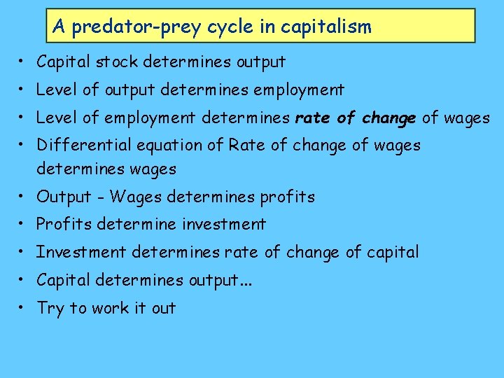
A predator-prey cycle in capitalism • Capital stock determines output • Level of output determines employment • Level of employment determines rate of change of wages • Differential equation of Rate of change of wages determines wages • Output - Wages determines profits • Profits determine investment • Investment determines rate of change of capital • Capital determines output. . . • Try to work it out

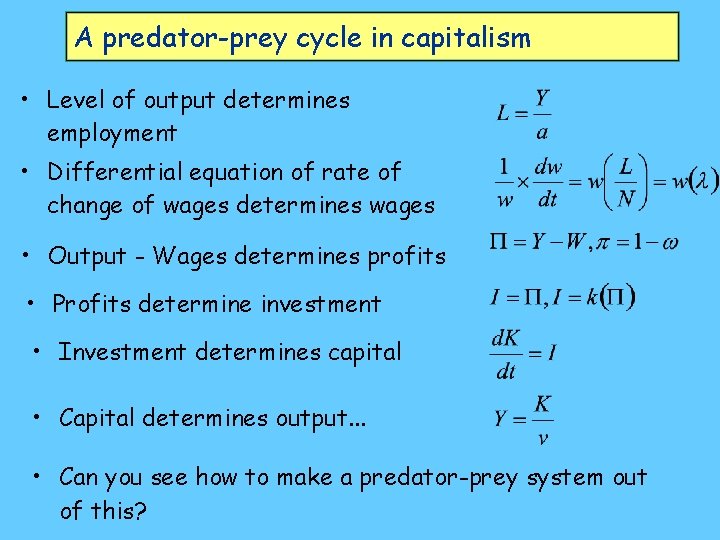
A predator-prey cycle in capitalism • Level of output determines employment • Differential equation of rate of change of wages determines wages • Output - Wages determines profits • Profits determine investment • Investment determines capital • Capital determines output. . . • Can you see how to make a predator-prey system out of this?

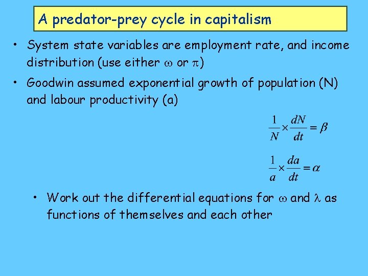
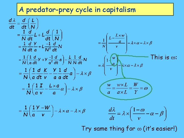
A predator-prey cycle in capitalism • System state variables are employment rate, and income distribution (use either or ) • Goodwin assumed exponential growth of population (N) and labour productivity (a) • Work out the differential equations for and as functions of themselves and each other

A predator-prey cycle in capitalism This is : Try same thing for (it’s easier!)

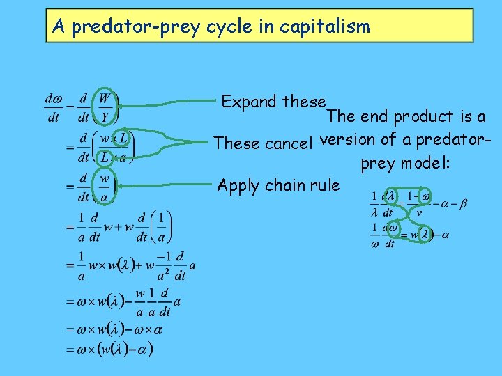
A predator-prey cycle in capitalism Expand these The end product is a These cancel version of a predatorprey model: Apply chain rule

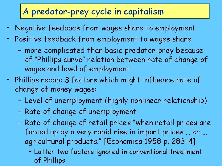
A predator-prey cycle in capitalism • Negative feedback from wages share to employment • Positive feedback from employment to wages share – more complicated than basic predator-prey because of “Phillips curve” relation between rate of change of wages and level of employment • Phillips recap: 3 factors which might influence rate of change of money wages: – Level of unemployment (highly nonlinear relationship) – Rate of change of unemployment – Rate of change of retail prices “when retail prices are forced up by a very rapid rise in import prices … or … agricultural products. ” [Economica 1958 p. 283 -4] • Latter two factors ignored in conventional treatment of Phillips

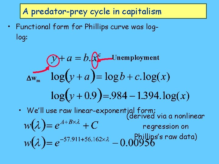
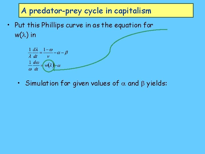
A predator-prey cycle in capitalism • Functional form for Phillips curve was loglog: Unemployment wm • We’ll use raw linear-exponential form: (derived via a nonlinear regression on Phillips’s raw data)

A predator-prey cycle in capitalism • Put this Phillips curve in as the equation for w( ) in • Simulation for given values of and yields:

A predator-prey cycle in capitalism • Goodwin/Marx model thus gives same basic cycle as biological predator-prey, but for wages share (income distribution) vs employment rather than fish vs sharks

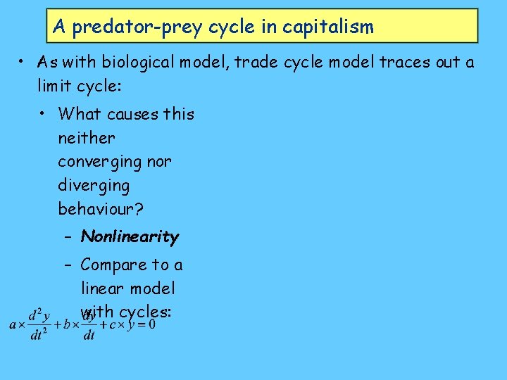
A predator-prey cycle in capitalism • As with biological model, trade cycle model traces out a limit cycle: • What causes this neither converging nor diverging behaviour? – Nonlinearity – Compare to a linear model with cycles:

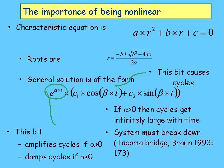
The importance of being nonlinear • Characteristic equation is • Roots are • General solution is of the form • This bit causes cycles • If >0 then cycles get infinitely large with time • This bit • System must break down (Tacoma bridge, Braun 1993: – amplifies cycles if >0 173) – damps cycles if <0

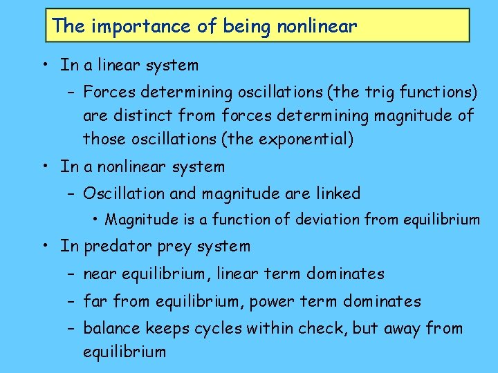
The importance of being nonlinear • In a linear system – Forces determining oscillations (the trig functions) are distinct from forces determining magnitude of those oscillations (the exponential) • In a nonlinear system – Oscillation and magnitude are linked • Magnitude is a function of deviation from equilibrium • In predator prey system – near equilibrium, linear term dominates – far from equilibrium, power term dominates – balance keeps cycles within check, but away from equilibrium

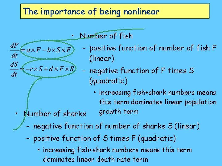
The importance of being nonlinear • Number of fish – positive function of number of fish F (linear) – negative function of F times S (quadratic) • Number of sharks • increasing fish+shark numbers means this term dominates linear population growth term – negative function of number of sharks S (linear) – positive function of S times F (quadratic) • increasing fish+shark numbers means this term dominates linear death rate term

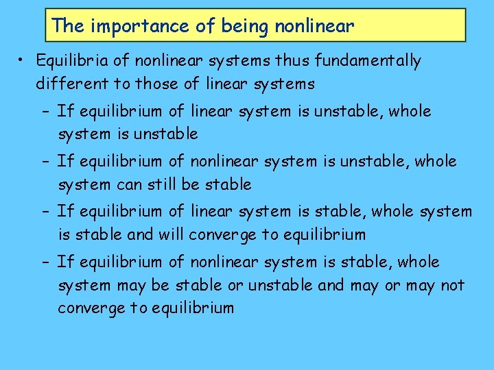
The importance of being nonlinear • Equilibria of nonlinear systems thus fundamentally different to those of linear systems – If equilibrium of linear system is unstable, whole system is unstable – If equilibrium of nonlinear system is unstable, whole system can still be stable – If equilibrium of linear system is stable, whole system is stable and will converge to equilibrium – If equilibrium of nonlinear system is stable, whole system may be stable or unstable and may or may not converge to equilibrium

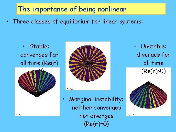
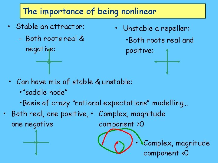
The importance of being nonlinear • Three classes of equilibrium for linear systems: • Stable: converges for all time (Re(r) < 0) • Unstable: diverges for all time (Re(r)>0) • Marginal instability: neither converges nor diverges (Re(r)=0)

The importance of being nonlinear • Stable an attractor: – Both roots real & negative: • Unstable a repeller: • Both roots real and positive: • Can have mix of stable & unstable: • “saddle node” • Basis of crazy “rational expectations” modelling… • Both real, one positive, • Complex, magnitude one negative component >0 • Complex, magnitude component <0

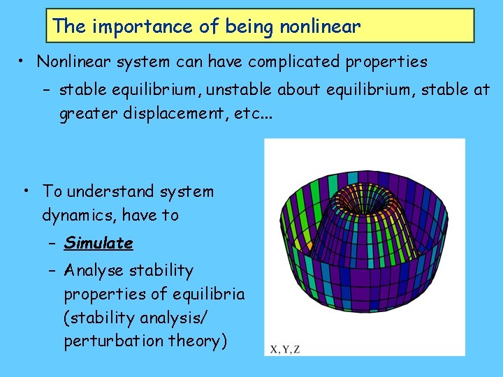
The importance of being nonlinear • Nonlinear system can have complicated properties – stable equilibrium, unstable about equilibrium, stable at greater displacement, etc. . . • To understand system dynamics, have to – Simulate – Analyse stability properties of equilibria (stability analysis/ perturbation theory)

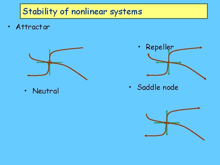
Stability of nonlinear systems • Simulation later today. . . • How to analyse the stability of a nonlinear equilibrium? – Linearise system about its equilibrium – Properties of complete nonlinear system will match those of linearised version about equilibrium point (but not far from it) – Can thus • identify equilibria of nonlinear system • characterise near equilibrium behaviour by behaviour of linear counterpart:

Stability of nonlinear systems • Attractor • Repeller • Neutral • Saddle node

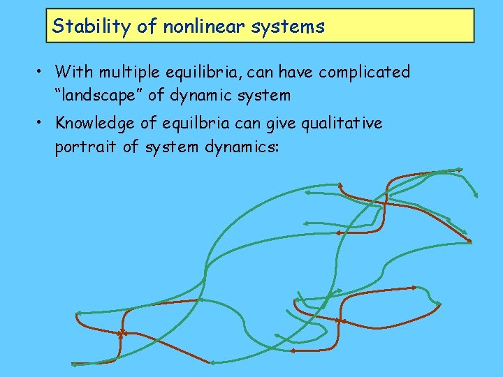
Stability of nonlinear systems • With multiple equilibria, can have complicated “landscape” of dynamic system • Knowledge of equilbria can give qualitative portrait of system dynamics:

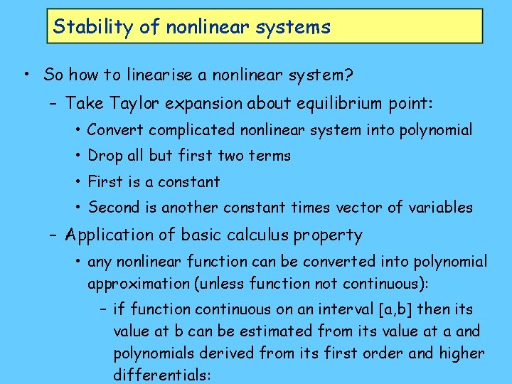
Stability of nonlinear systems • So how to linearise a nonlinear system? – Take Taylor expansion about equilibrium point: • Convert complicated nonlinear system into polynomial • Drop all but first two terms • First is a constant • Second is another constant times vector of variables – Application of basic calculus property • any nonlinear function can be converted into polynomial approximation (unless function not continuous): – if function continuous on an interval [a, b] then its value at b can be estimated from its value at a and polynomials derived from its first order and higher differentials:

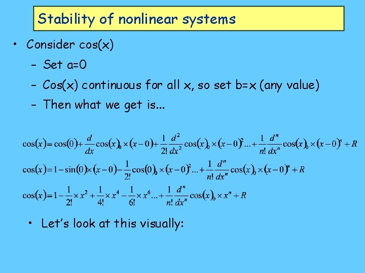
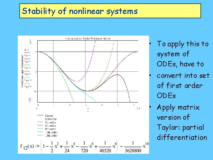
Stability of nonlinear systems • Consider cos(x) – Set a=0 – Cos(x) continuous for all x, so set b=x (any value) – Then what we get is. . . • Let’s look at this visually:

Stability of nonlinear systems • To apply this to system of ODEs, have to • convert into set of first order ODEs • Apply matrix version of Taylor: partial differentiation

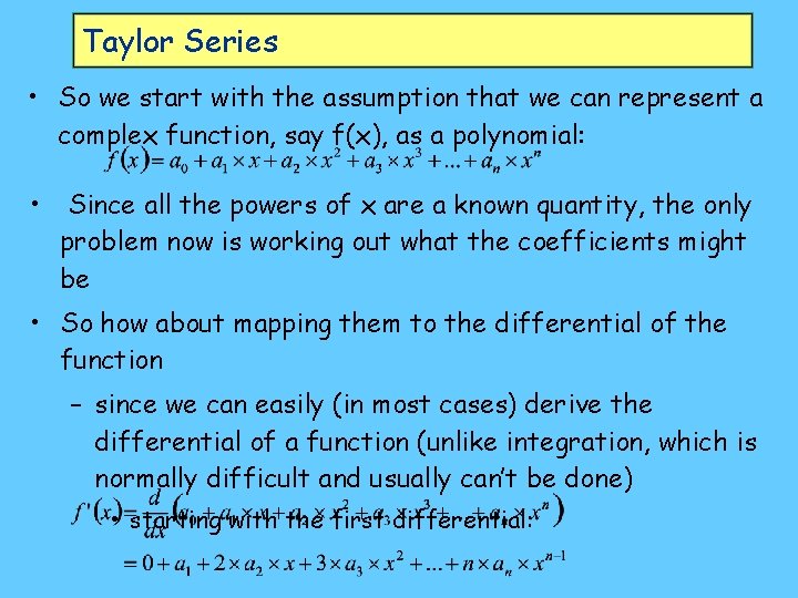
Taylor Series • Taylor Series are a delightful example of the application of the basic rules of mathematics: – what have we got that we don’t want? • A complex equation (sin, cos, exponential, log, etc. ) that we can’t easily numerically estimate – what do we want that we can put in? • something simple--like a polynomial – keep it balanced • So the basic question is “can we estimate a difficult function using something simple like a polynomial? ” • The answer is “let’s just assume the answer is yes and see what falls out

Taylor Series • So we start with the assumption that we can represent a complex function, say f(x), as a polynomial: • Since all the powers of x are a known quantity, the only problem now is working out what the coefficients might be • So how about mapping them to the differential of the function – since we can easily (in most cases) derive the differential of a function (unlike integration, which is normally difficult and usually can’t be done) • starting with the first differential:

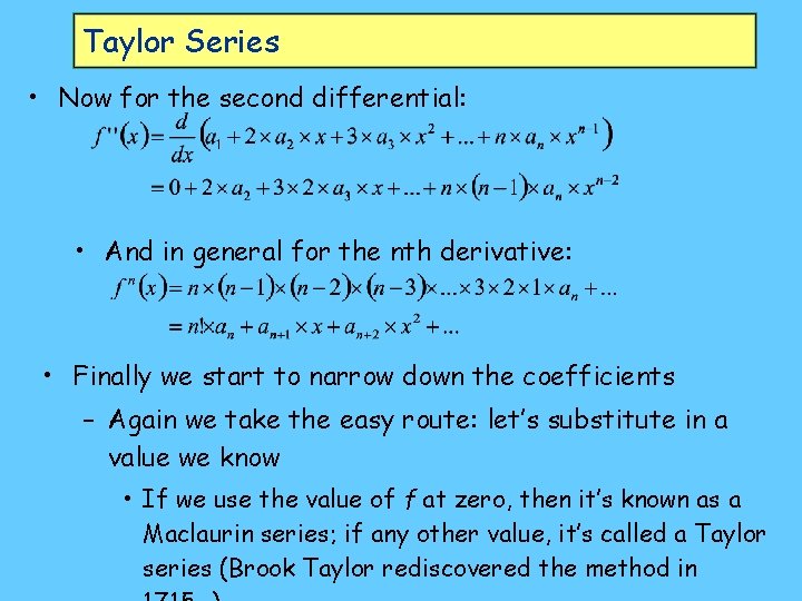
Taylor Series • Now for the second differential: • And in general for the nth derivative: • Finally we start to narrow down the coefficients – Again we take the easy route: let’s substitute in a value we know • If we use the value of f at zero, then it’s known as a Maclaurin series; if any other value, it’s called a Taylor series (Brook Taylor rediscovered the method in

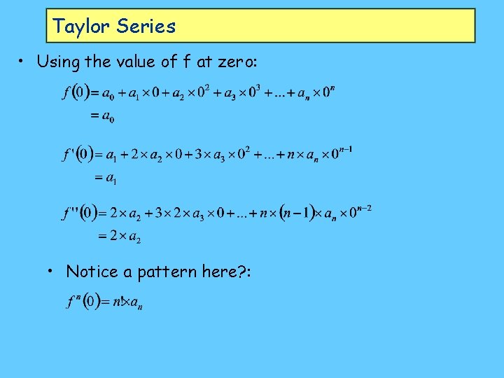
Taylor Series • Using the value of f at zero: • Notice a pattern here? :

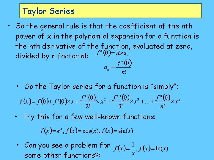
Taylor Series • So the general rule is that the coefficient of the nth power of x in the polynomial expansion for a function is the nth derivative of the function, evaluated at zero, divided by n factorial: • So the Taylor series for a function is “simply”: • Try this for a few well-known functions: • Can you see a problem for some other functions? :

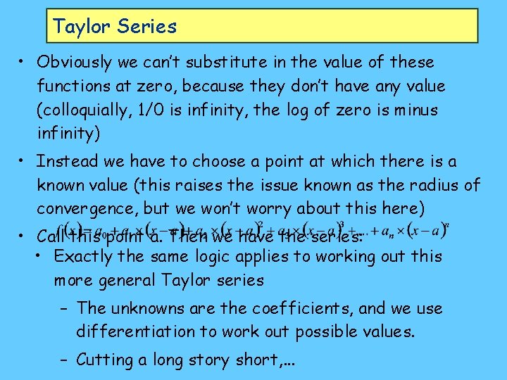
Taylor Series • Obviously we can’t substitute in the value of these functions at zero, because they don’t have any value (colloquially, 1/0 is infinity, the log of zero is minus infinity) • Instead we have to choose a point at which there is a known value (this raises the issue known as the radius of convergence, but we won’t worry about this here) • Call this point a. Then we have the series: • Exactly the same logic applies to working out this more general Taylor series – The unknowns are the coefficients, and we use differentiation to work out possible values. – Cutting a long story short, . . .

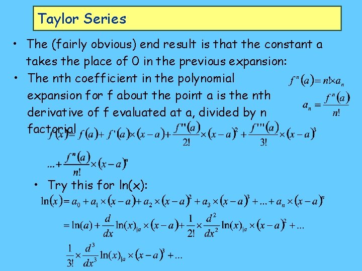
Taylor Series • The (fairly obvious) end result is that the constant a takes the place of 0 in the previous expansion: • The nth coefficient in the polynomial expansion for f about the point a is the nth derivative of f evaluated at a, divided by n factorial • Try this for ln(x):

Taylor Series • The differentials of ln are: • We can substitute to give, in complete detail:

Taylor Series • Try this using a=1, at which point ln(1)=0:

Taylor Series • We get: • This works for x>0 (since ln of a negative number is not defined); but it doesn’t converge very well (for reasons we won’t go into). Points other than 1 converge

Taylor Series • So why are we bothering with all this stuff? – The bad news: to work out stability properties, we have to linearise a nonlinear system of ODEs in vicinity of (non-trivial, hence not zero) equilibrium point • More bad news: we have to apply the matrix equivalent of a Taylor series, which means powers of matrices, etc. – The good news: since we’re trying to linearise the system, all we’re interested in are the first two terms: • The first matrix of constants, which since it’s based on the equilibrium point of the system will be a matrix of zeros • The second matrix of constants, which simply involves the first differentials of the system and multiplies the vector of variables

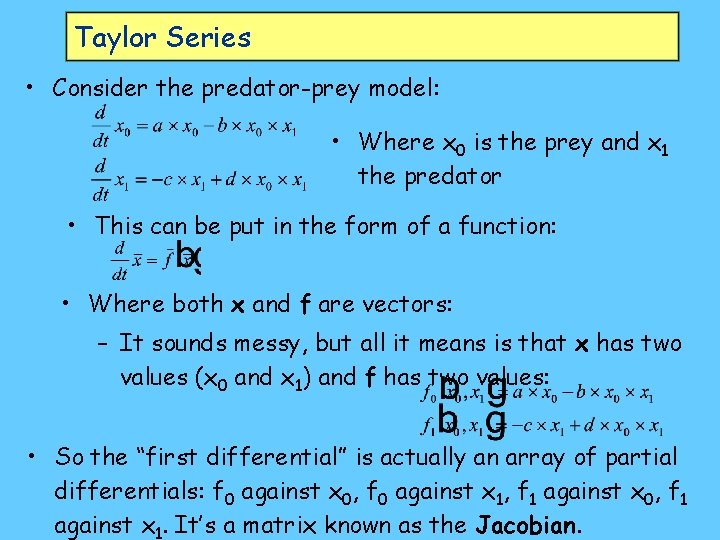
Taylor Series • Consider the predator-prey model: • Where x 0 is the prey and x 1 the predator • This can be put in the form of a function: • Where both x and f are vectors: – It sounds messy, but all it means is that x has two values (x 0 and x 1) and f has two values: • So the “first differential” is actually an array of partial differentials: f 0 against x 0, f 0 against x 1, f 1 against x 0, f 1 against x 1. It’s a matrix known as the Jacobian.

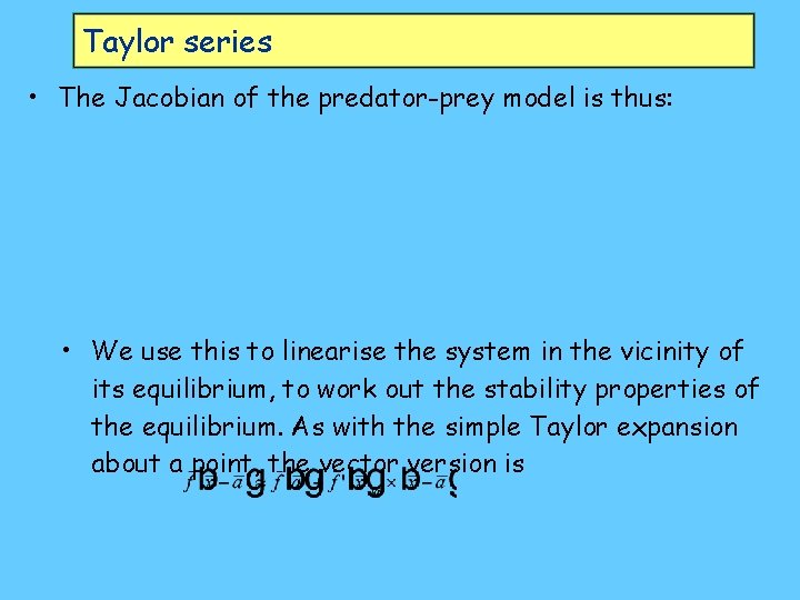
Taylor series • The Jacobian of the predator-prey model is thus: • We use this to linearise the system in the vicinity of its equilibrium, to work out the stability properties of the equilibrium. As with the simple Taylor expansion about a point, the vector version is

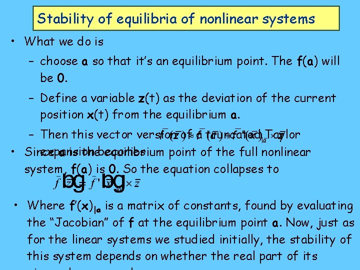
Stability of equilibria of nonlinear systems • What we do is – choose a so that it’s an equilibrium point. The f(a) will be 0. – Define a variable z(t) as the deviation of the current position x(t) from the equilibrium a. – Then this vector version of a truncated Taylor expansion • Since a is thebecomes equilibrium point of the full nonlinear system, f(a) is 0. So the equation collapses to • Where f’(x)|a is a matrix of constants, found by evaluating the “Jacobian” of f at the equilibrium point a. Now, just as for the linear systems we studied initially, the stability of this system depends on whether the real part of its

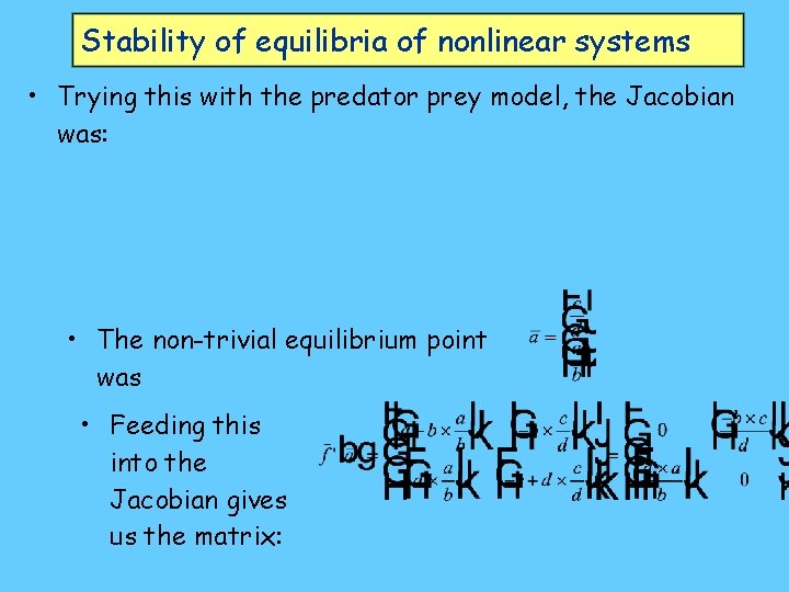
Stability of equilibria of nonlinear systems • Trying this with the predator prey model, the Jacobian was: • The non-trivial equilibrium point was • Feeding this into the Jacobian gives us the matrix:

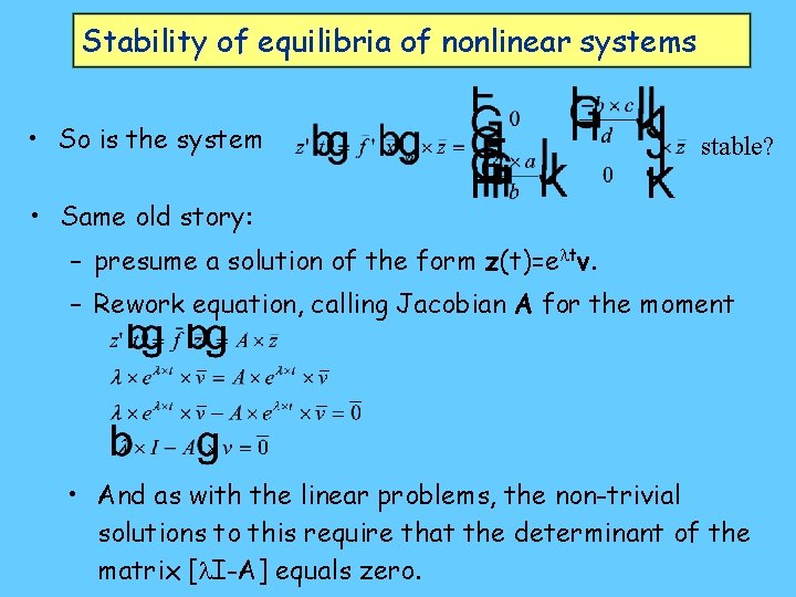
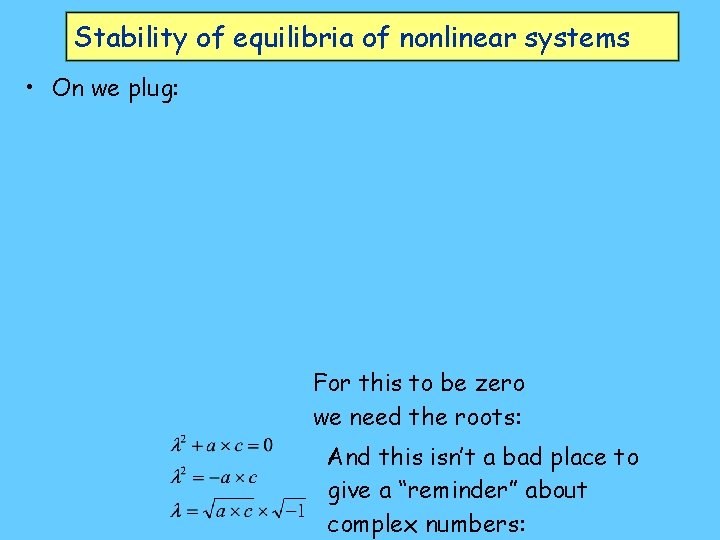
Stability of equilibria of nonlinear systems • So is the system stable? • Same old story: – presume a solution of the form z(t)=e tv. – Rework equation, calling Jacobian A for the moment • And as with the linear problems, the non-trivial solutions to this require that the determinant of the matrix [ I-A] equals zero.

Stability of equilibria of nonlinear systems • On we plug: For this to be zero we need the roots: And this isn’t a bad place to give a “reminder” about complex numbers:

Complex numbers • These are numbers which have a real component (as you’re used to) and a component multiplied by the square root of minus one • They were invented because without them, many quadratics did not have a solution--like the one we’re looking at now. • The reason they matter to us in dynamic analysis is because they have the effect of generating cycles in mathematical models of real systems • The reason they do this is because there is a very exact correspondence between exponentials, complex numbers, and the trigonometric functions sin and cos. • This can be proven (don’t ask me now!) but it can also be

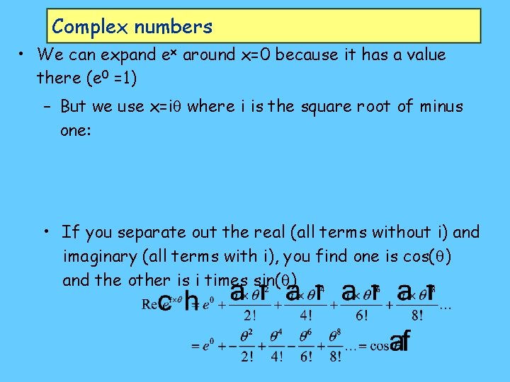
Complex numbers • We can expand ex around x=0 because it has a value there (e 0 =1) – But we use x=i where i is the square root of minus one: • If you separate out the real (all terms without i) and imaginary (all terms with i), you find one is cos( ) and the other is i times sin( )

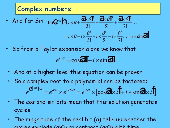
Complex numbers • And for Sin: • So from a Taylor expansion alone we know that • And at a higher level this equation can be proven • So a complex root to a polynomial can be factored: • The cos and sin bits mean that this solution generates cycles • The magnitude of the real bit (a) tells us whether the

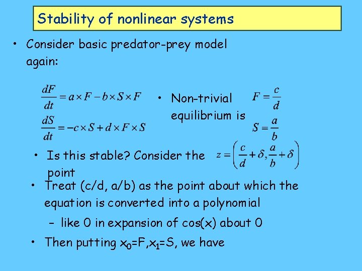
Stability of nonlinear systems • Consider basic predator-prey model again: • Non-trivial equilibrium is • Is this stable? Consider the point • Treat (c/d, a/b) as the point about which the equation is converted into a polynomial – like 0 in expansion of cos(x) about 0 • Then putting x 0=F, x 1=S, we have

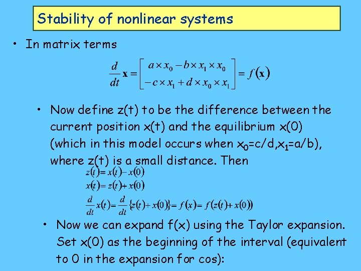
Stability of nonlinear systems • In matrix terms • Now define z(t) to be the difference between the current position x(t) and the equilibrium x(0) (which in this model occurs when x 0=c/d, x 1=a/b), where z(t) is a small distance. Then • Now we can expand f(x) using the Taylor expansion. Set x(0) as the beginning of the interval (equivalent to 0 in the expansion for cos):

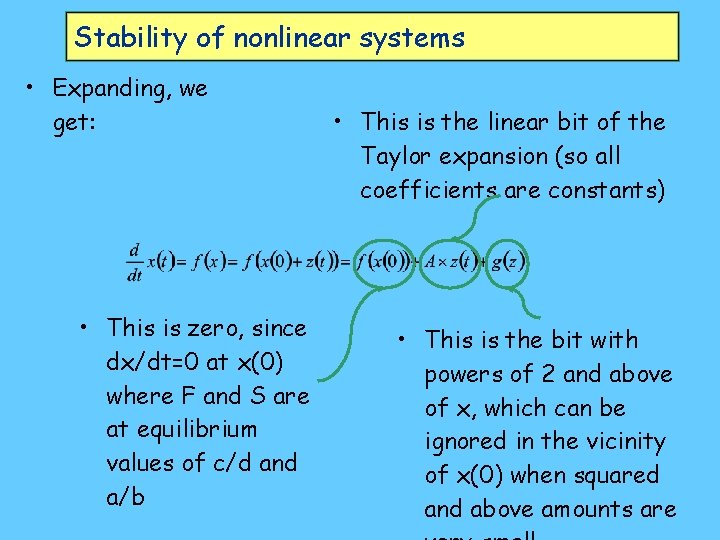
Stability of nonlinear systems • Expanding, we get: • This is zero, since dx/dt=0 at x(0) where F and S are at equilibrium values of c/d and a/b • This is the linear bit of the Taylor expansion (so all coefficients are constants) • This is the bit with powers of 2 and above of x, which can be ignored in the vicinity of x(0) when squared and above amounts are

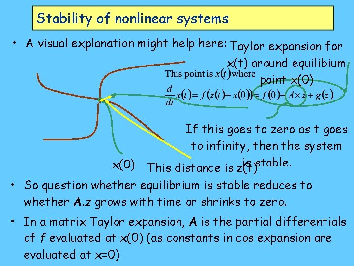
Stability of nonlinear systems • A visual explanation might help here: Taylor expansion for x(t) around equilibium point x(0) If this goes to zero as t goes to infinity, then the system is stable. This distance is z(t) • So question whether equilibrium is stable reduces to whether A. z grows with time or shrinks to zero. • In a matrix Taylor expansion, A is the partial differentials of f evaluated at x(0) (as constants in cos expansion are evaluated at x=0)

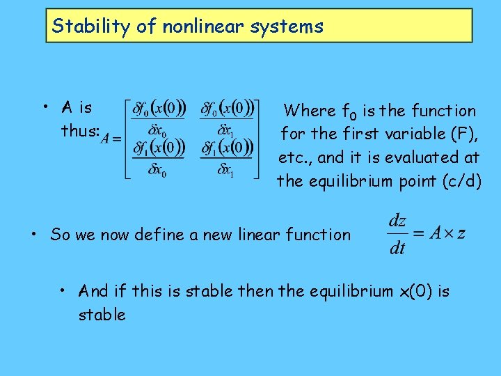
Stability of nonlinear systems • A is thus: Where f 0 is the function for the first variable (F), etc. , and it is evaluated at the equilibrium point (c/d) • So we now define a new linear function • And if this is stable then the equilibrium x(0) is stable

Stability of nonlinear systems • What is A for our example of a predator-prey system?

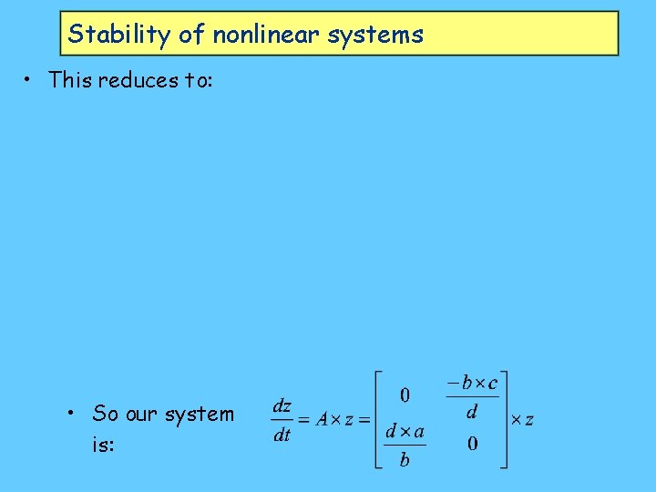
Stability of nonlinear systems • This reduces to: • So our system is:

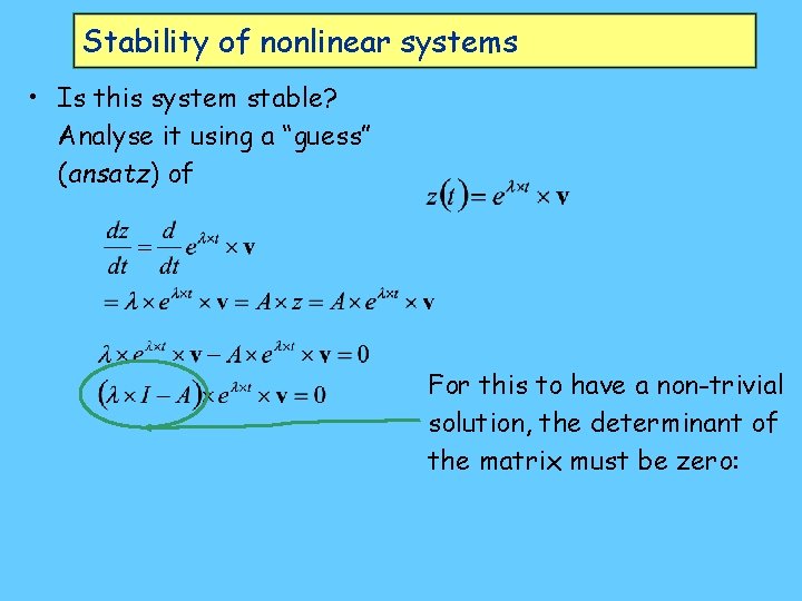
Stability of nonlinear systems • Is this system stable? Analyse it using a “guess” (ansatz) of For this to have a non-trivial solution, the determinant of the matrix must be zero:

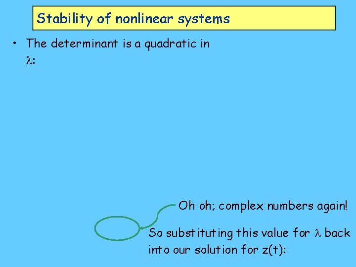
Stability of nonlinear systems • The determinant is a quadratic in : Oh oh; complex numbers again! So substituting this value for back into our solution for z(t):

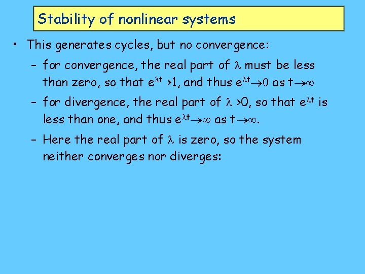
Stability of nonlinear systems • This generates cycles, but no convergence: – for convergence, the real part of must be less than zero, so that e t >1, and thus e t as t – for divergence, the real part of >0, so that e t is less than one, and thus e t as t . – Here the real part of is zero, so the system neither converges nor diverges:

Stability of nonlinear systems • This explains closed limit cycle behaviour of Goodwin model – Many other behaviours possible for nonlinear model • Technique works in vicinity of equilibrium, but doesn’t tell you anything about behaviour away from equilibrium • To characterise overall stability of nonlinear system, techniques used which “explore parameter space” – How stable is system for varying values of constants, different initial conditions? • Lyapunov exponents (large-scale eigenvalue analysis), etc. • Can also simulate, as shown earlier • Combination of two needed to fully characterise system

Simulation • Numerical simulation of analytically insoluble ODEs/PDEs relies upon – Approximation methods • simplest Euler method • more complex (and accurate) Runge-Kutta algorithm • based on Taylor-style logic – next value of function can be estimated from current value plus derivatives evaluated at current value – “ -shadowing” hypothesis for chaotic systems • Despite “sensitive dependence on initial conditions”, simulation can be guaranteed to shadow an actual trajectory of a system, though not the one intended to be simulated

Simulation • Two broad classes of simulation tools – “Top down” • system specified as – set of ODEs/PDEs – system of flowcharts – “Bottom up” • characteristics of agents in such a system described in computer program • environment of system constructed as “experience space” for agents • system run as “virtual world”

Simulation • “Top Down” programs – ODE/PDE approach • Mathematica, Mathcad, Maple, Matlab – Flowchart approach • Matlab/Simulink, Vissim, IThink, Vensim • “Bottom up” programs – Few commercial versions as yet (Sim. City? ) – Many research programs, some public domain: Swarm, Terra, Ecolab • Illustration of both top down approaches for predatorprey model:

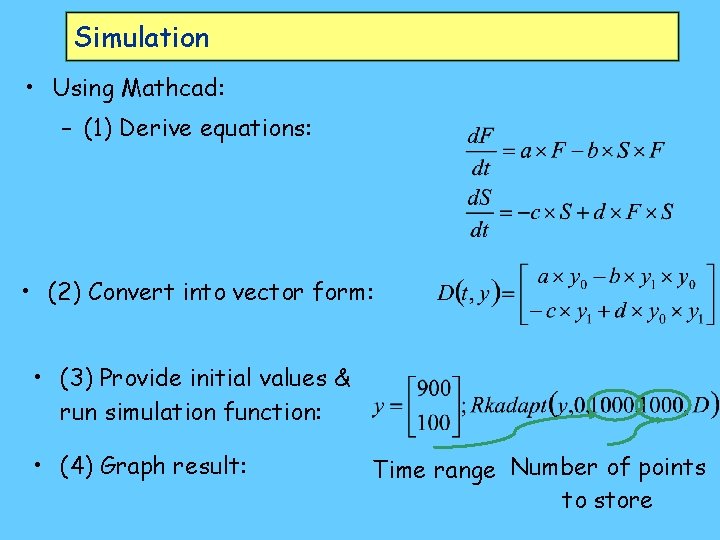
Simulation • Using Mathcad: – (1) Derive equations: • (2) Convert into vector form: • (3) Provide initial values & run simulation function: • (4) Graph result: Time range Number of points to store

Simulation • (5) Run simulations with varying parameters many times for phase space analysis (Lyapunov, etc. ), production of phase portraits. . .

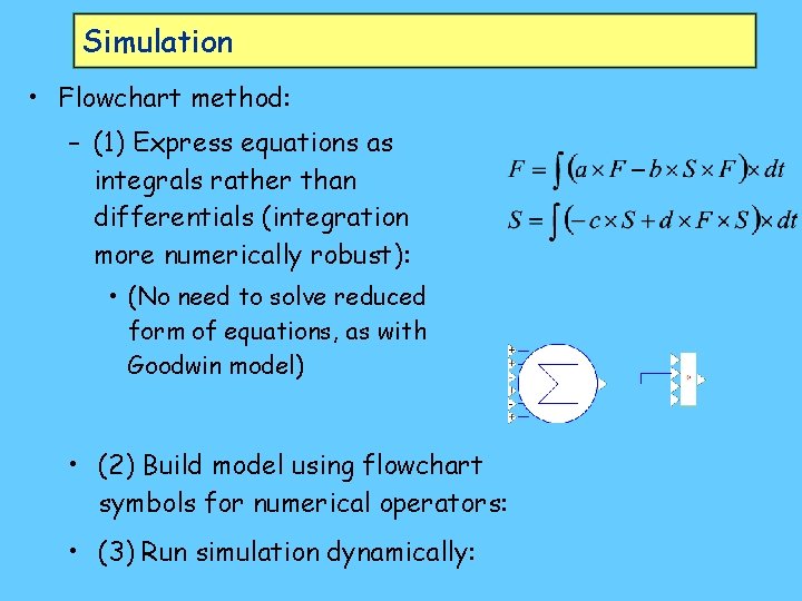
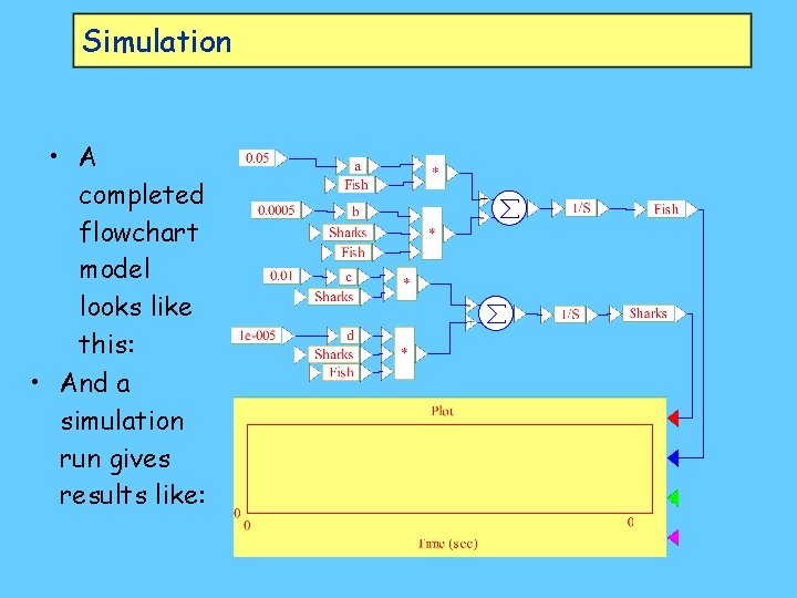
Simulation • Flowchart method: – (1) Express equations as integrals rather than differentials (integration more numerically robust): • (No need to solve reduced form of equations, as with Goodwin model) • (2) Build model using flowchart symbols for numerical operators: • (3) Run simulation dynamically:

Simulation • A completed flowchart model looks like this: • And a simulation run gives results like:

Simulation

Next Week • Derive a model of the “Dual Price Level Hypothesis” • Simulate it and discuss results