HighOrder Adaptive and Parallel Discontinuous Galerkin Methods for

High-Order Adaptive and Parallel Discontinuous Galerkin Methods for Hyperbolic Conservation Laws J. E. Flaherty, L. Krivodonova, J. F. Remacle, and M. S. Shephard Scientific Computation Research Center

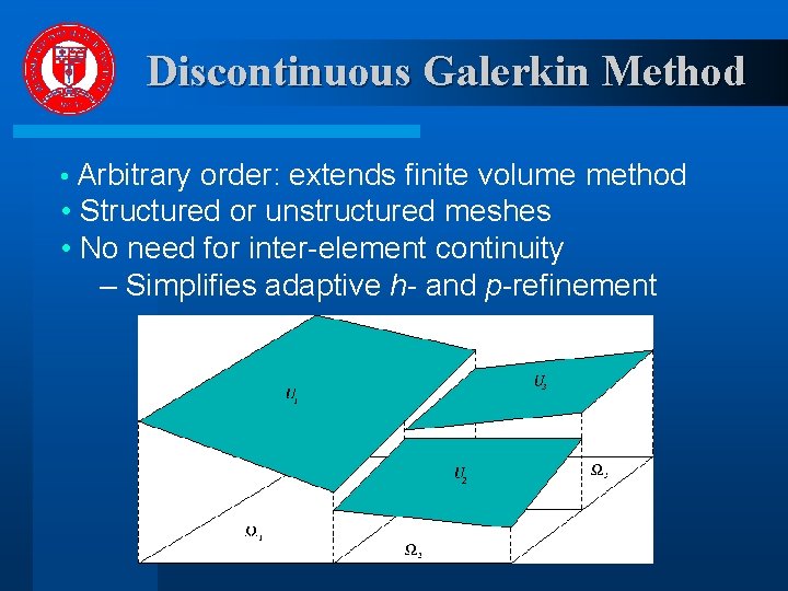
Discontinuous Galerkin Method • Arbitrary order: extends finite volume method • Structured or unstructured meshes • No need for inter-element continuity – Simplifies adaptive h- and p-refinement

Discontinuous Galerkin Method • Face-based communication – Simplifies parallel computation • Sharp capturing of discontinuities • Element level conservation • A posteriori error estimates

Discontinuous Galerkin Method • Face-based communication – Simplifies parallel computation • Sharp capturing of discontinuities • Element level conservation • A posteriori error estimates However: • More mesh unknowns than FEM for same order • Possibly OK with parallel computation • Monotonicty control (limiting) is difficult

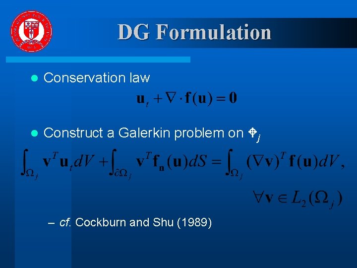
DG Formulation l Conservation law l Construct a Galerkin problem on j – cf. Cockburn and Shu (1989)

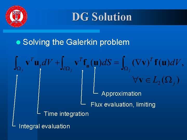
DG Solution l Solving the Galerkin problem Approximation Flux evaluation, limiting Time integration Integral evaluation

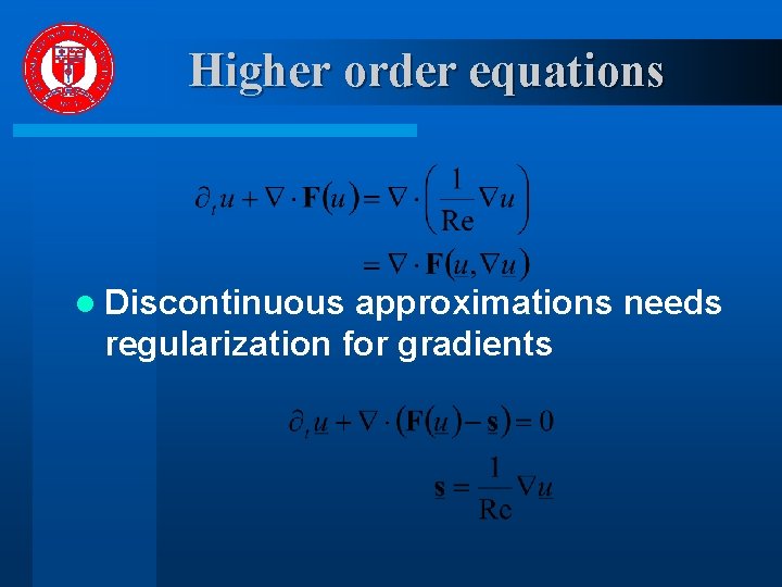
Higher order equations l Discontinuous approximations needs regularization for gradients

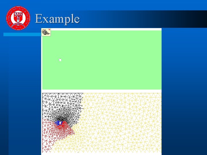
Example

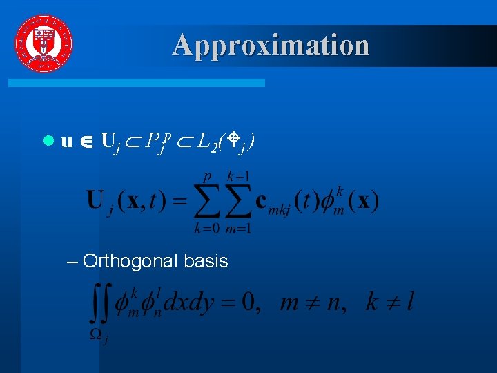
Approximation lu Uj Pjp L 2( j ) – Orthogonal basis

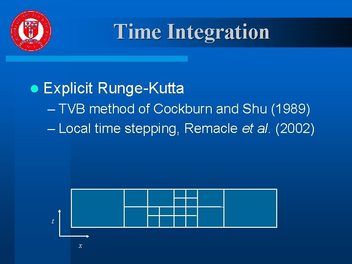
Time Integration l Explicit Runge-Kutta – TVB method of Cockburn and Shu (1989) – Local time stepping, Remacle et al. (2002) t x

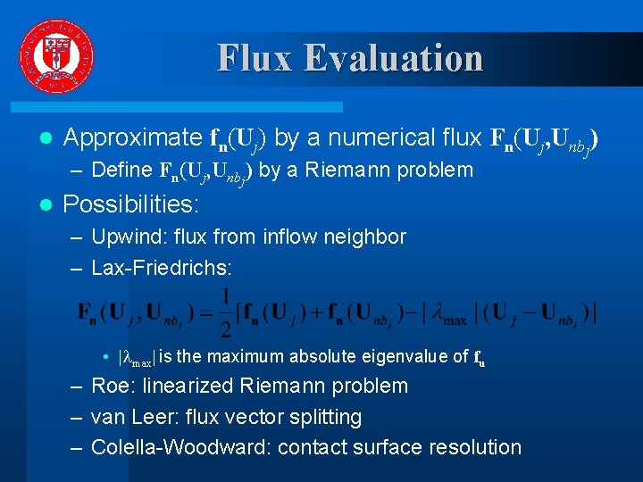
Flux Evaluation l Approximate fn(Uj) by a numerical flux Fn(Uj, Unbj) – Define Fn(Uj, Unbj) by a Riemann problem l Possibilities: – Upwind: flux from inflow neighbor – Lax-Friedrichs: • | max| is the maximum absolute eigenvalue of fu – Roe: linearized Riemann problem – van Leer: flux vector splitting – Colella-Woodward: contact surface resolution

Limiting: suppress spurious oscillations when p > 0 while maintaining order – Slope limiter: Cockburn and Shu (1989) – Curvature limiter: Barth (1990) – Moment limiter: Biswas et al. (1994) – Filtering: Gottlieb et al. (1999) l No robust procedures for multi-dimensional situations l

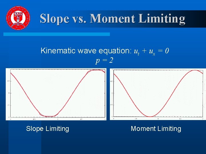
Slope vs. Moment Limiting Kinematic wave equation: ut + ux = 0 p=2 Slope Limiting Moment Limiting

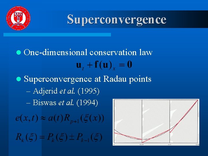
Superconvergence l One-dimensional conservation law l Superconvergence at Radau points – Adjerid et al. (1995) – Biswas et al. (1994)

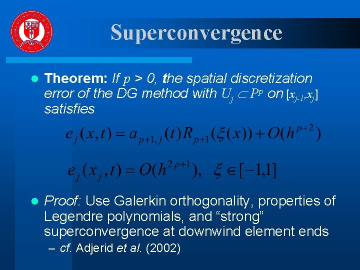
Superconvergence l Theorem: If p > 0, the spatial discretization error of the DG method with Uj Pp on [xj-1, xj] satisfies l Proof: Use Galerkin orthogonality, properties of Legendre polynomials, and “strong” superconvergence at downwind element ends – cf. Adjerid et al. (2002)

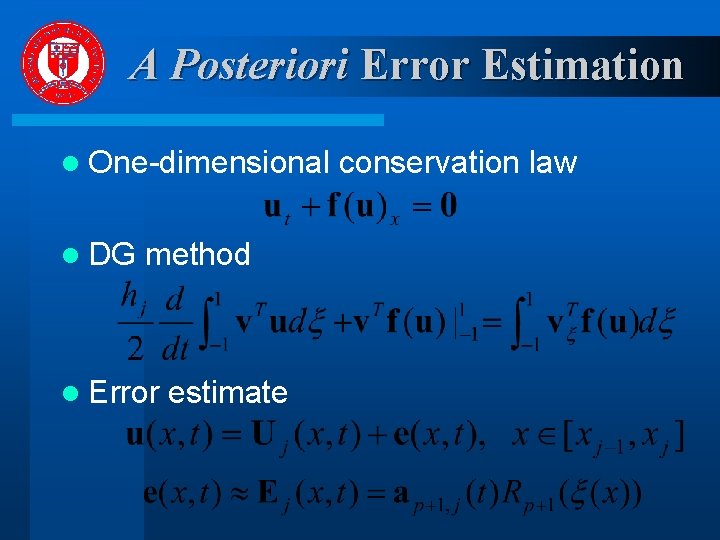
A Posteriori Error Estimation l One-dimensional l DG method l Error estimate conservation law

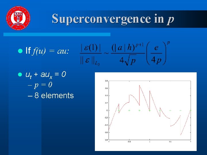
Superconvergence in p l If l f(u) = au: ut + aux = 0 –p=0 – 8 elements

Superconvergence in p l If l f(u) = au: ut + aux = 0 –p=1 – 8 elements

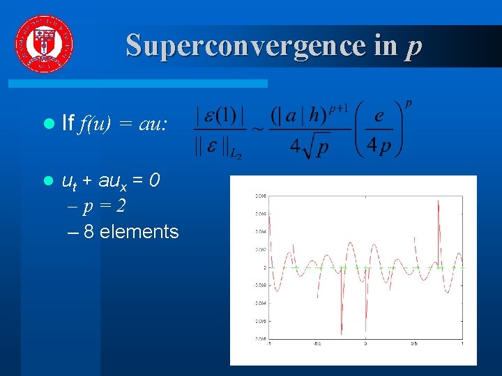
Superconvergence in p l If l f(u) = au: ut + aux = 0 –p=2 – 8 elements

Superconvergence in p l If l f(u) = au: ut + aux = 0 –p=3 – 8 elements

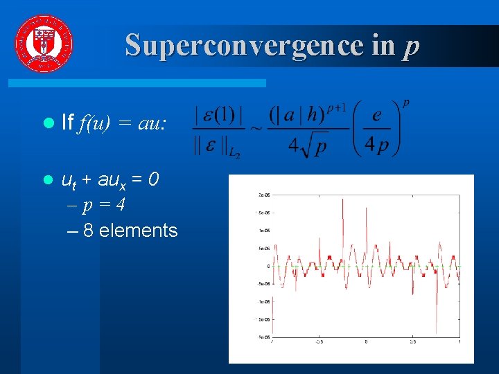
Superconvergence in p l If l f(u) = au: ut + aux = 0 –p=4 – 8 elements

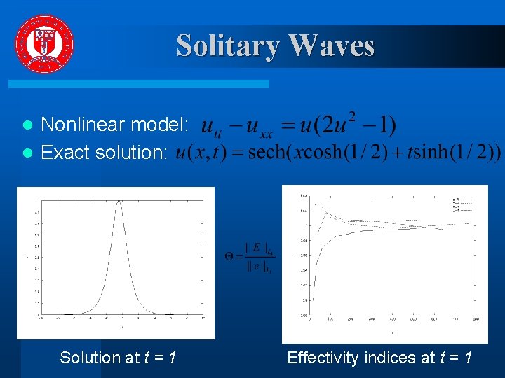
Solitary Waves Nonlinear model: l Exact solution: l Solution at t = 1 Effectivity indices at t = 1

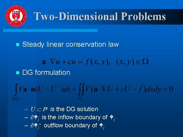
Two-Dimensional Problems l Steady linear conservation law l DG formulation – U Pp is the DG solution – j- is the inflow boundary of j – j+ outflow boundary of j

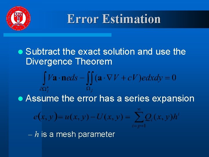
Error Estimation l Subtract the exact solution and use the Divergence Theorem l Assume the error has a series expansion – h is a mesh parameter

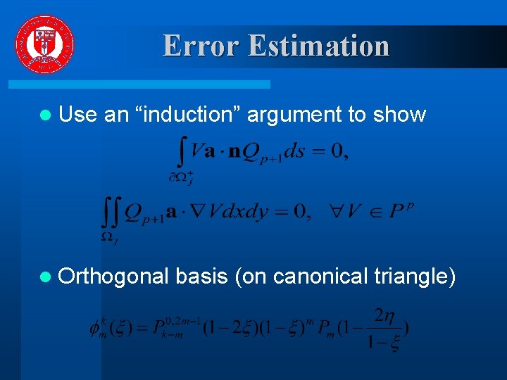
Error Estimation l Use an “induction” argument to show l Orthogonal basis (on canonical triangle)

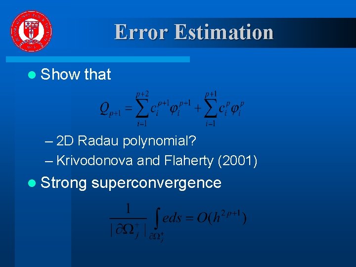
Error Estimation l Show that – 2 D Radau polynomial? – Krivodonova and Flaherty (2001) l Strong superconvergence

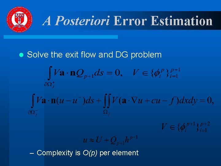
A Posteriori Error Estimation l Solve the exit flow and DG problem – Complexity is O(p) per element

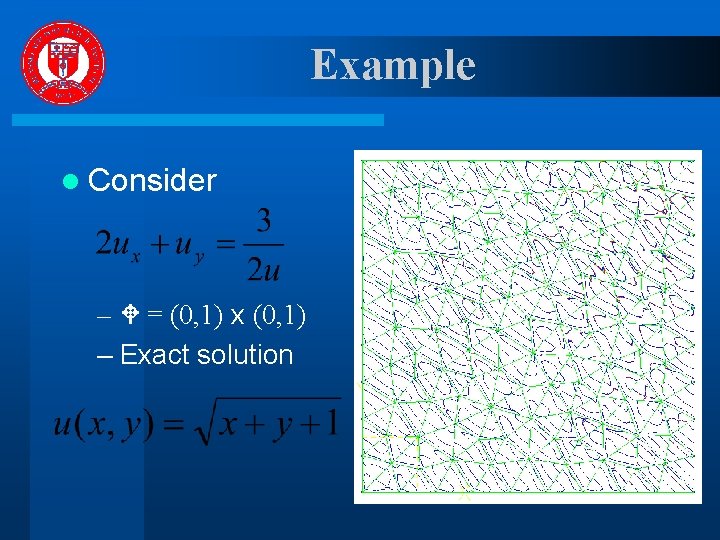
Example l Consider – = (0, 1) x (0, 1) – Exact solution

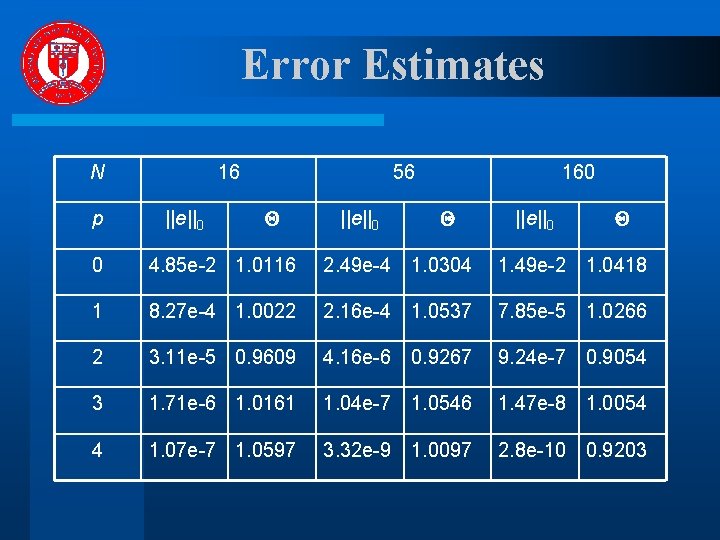
Error Estimates N p 16 ||e||0 56 ||e||0 160 ||e||0 0 4. 85 e-2 1. 0116 2. 49 e-4 1. 0304 1. 49 e-2 1. 0418 1 8. 27 e-4 1. 0022 2. 16 e-4 1. 0537 7. 85 e-5 1. 0266 2 3. 11 e-5 0. 9609 4. 16 e-6 0. 9267 9. 24 e-7 0. 9054 3 1. 71 e-6 1. 0161 1. 04 e-7 1. 0546 1. 47 e-8 1. 0054 4 1. 07 e-7 1. 0597 3. 32 e-9 1. 0097 2. 8 e-10 0. 9203

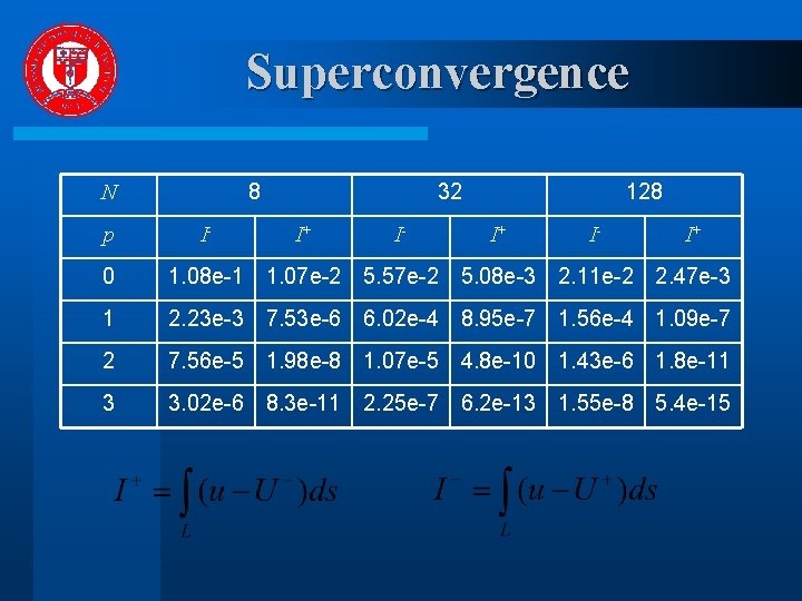
Superconvergence 8 N p I- 32 I+ I- 128 I+ I- I+ 0 1. 08 e-1 1. 07 e-2 5. 57 e-2 5. 08 e-3 2. 11 e-2 2. 47 e-3 1 2. 23 e-3 7. 53 e-6 6. 02 e-4 8. 95 e-7 1. 56 e-4 1. 09 e-7 2 7. 56 e-5 1. 98 e-8 1. 07 e-5 4. 8 e-10 1. 43 e-6 1. 8 e-11 3 3. 02 e-6 8. 3 e-11 2. 25 e-7 6. 2 e-13 1. 55 e-8 5. 4 e-15

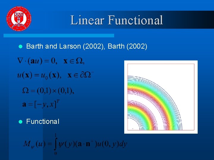
Linear Functional l Barth and Larson (2002), Barth (2002) l Functional

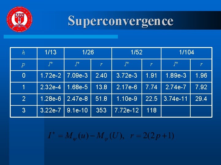
Superconvergence h 1/13 p I+ 1/26 I+ 1/52 1/104 r I+ r 0 1. 72 e-2 7. 09 e-3 2. 40 3. 72 e-3 1. 91 1. 89 e-3 1. 96 1 2. 32 e-4 1. 68 e-5 13. 8 2. 17 e-6 7. 74 2. 74 e-7 7. 92 2 1. 28 e-6 2. 47 e-8 51. 8 1. 10 e-9 22. 5 3. 74 e-11 29. 4 3 3. 22 e-7 9. 1 e-10 353 7. 72 e-12 118

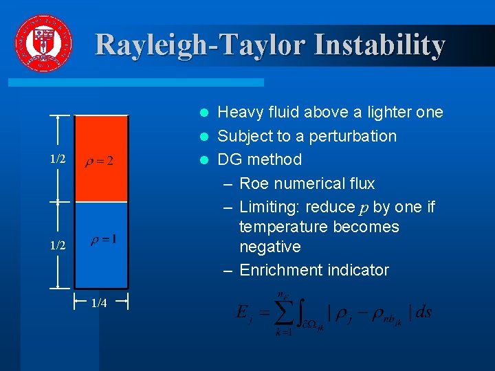
Rayleigh-Taylor Instability Heavy fluid above a lighter one l Subject to a perturbation l DG method – Roe numerical flux – Limiting: reduce p by one if temperature becomes negative – Enrichment indicator l 1/2 1/4

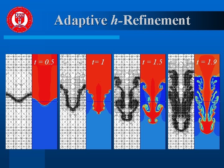
Adaptive h-Refinement t = 0. 5 t= 1 t = 1. 5 t = 1. 9

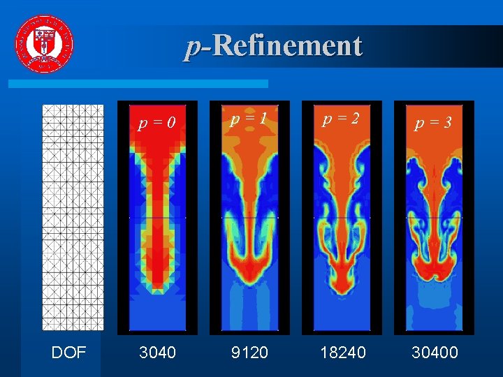
p-Refinement DOF p=0 p=1 p=2 p=3 3040 9120 18240 30400

Vortex sheet

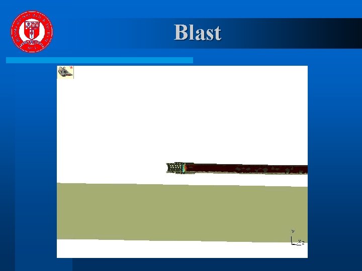
Blast

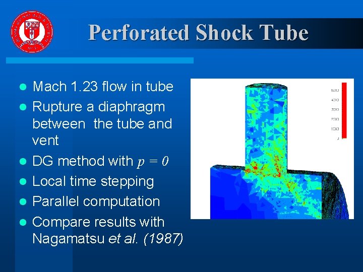
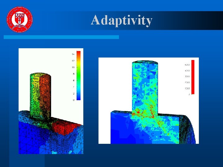
Perforated Shock Tube l l l Mach 1. 23 flow in tube Rupture a diaphragm between the tube and vent DG method with p = 0 Local time stepping Parallel computation Compare results with Nagamatsu et al. (1987)

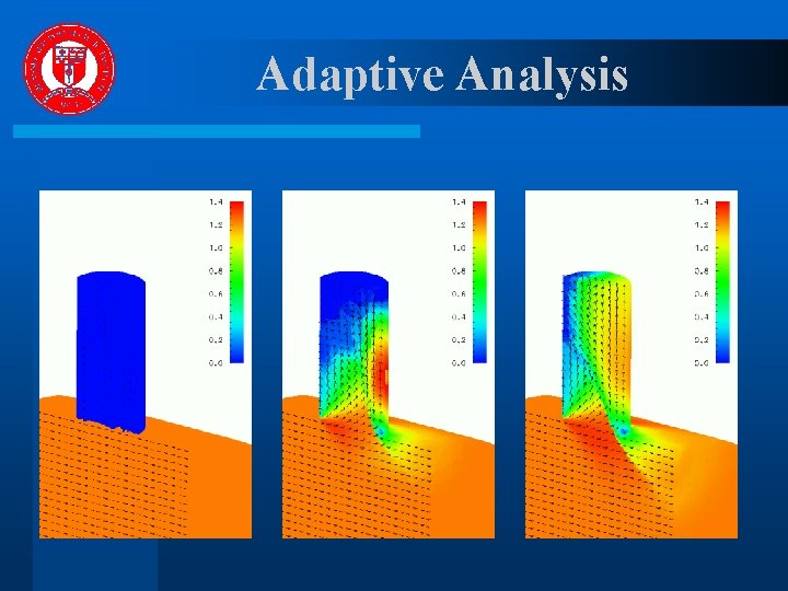
Adaptive Analysis

Adaptivity

Discussion l Stabilization (limiting) – Unstructured meshes Viscosity: Navier-Stokes equations l Implicit time integration l – Space-time DG method l A posteriori error estimation – Discontinuities – Space-time coordination – Multi-dimensional superconvergence? l Adaptive strategies – Optimal enrichment (with parallel computation)