Genes in populations Xuhua Xia xxiauottawa ca http

Genes in populations Xuhua Xia xxia@uottawa. ca http: //dambe. bio. uottawa. ca

Outline • Experimental methods for detecting alleles – Protein electrophoresis (different proteins could have the same migration speed) – DNA: • Tandom repeats and length polymorphism – variable number tandem repeat (VNTR or minisatellites): each unit is six bases or longer – Short tandem repeats (STRs or microsatellite), each unit is six bases or shorter • Single nucleotide polymorphism (SNP) • Application of alleles as genetic marks • Effect of selection, mutation and drift on allele frequencies Xuhua Xia Slide 2

MUTATIONS and POLYMORPHISMS • Alleles • alternative forms of a gene (or DNA sequence) at a particular locus (chromosomal site) • frequency in population determined by natural selection and random genetic drift • a rare allele (e. g. , <2%) is called a mutant allele in contrast to the common allele referred to as wild type, but a mutant can increase in frequency and become wild type • Polymorphisms • two or more natural variants (alleles, phenotypes, homologous sequences) which occur at measurable frequencies in a population • Allele fixed: allele frequency = 1. A substitution occurs when a mutant increases in frequency and becomes fixed • Allele lost: allele frequency = 0.

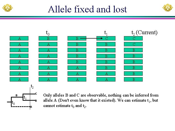
Conceptual & operational definitions • Allele fixed: allele frequency = 1 (Every allele in the population descends from that allele). • Allele lost: allele frequency = 0 (No one in the population descends from the allele). • Suppose a population with allele A fixed. At time t 0 an advantageous allele B originated and was on its way towards fixation, but one copy of B, at time t 1 mutated into another allele C which was also advantageous. Suppose that allele A was lost at time t 2, can we say that allele B is fixed because all existing alleles descend from it? • If B and C are indistinguishable, then they would be considered as the same allele and indeed it is fixed; if they are distinguishable, then they are not fixed.

Allele fixed and lost t 0 A t 1 t 2 (Current) B B A A B B C A A B B B A A A A B C C t 2 B t 0 C t 1 B A Only alleles B and C are observable, nothing can be inferred from allele A (Don't even know that it existed). We can estimate t 1, but cannot estimate t 0 and t 2.

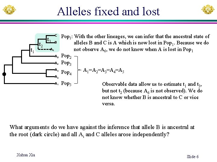
Alleles fixed and lost t 1 t 2 t 3 C B A 6 A 5 A 4 A 3 A 2 A 1 Pop 1: With the other lineages, we can infer that the ancestral state of alleles B and C is A which is now lost in Pop 1. Because we do not observe A 6, we do not know when A is lost in Pop 1 Pop 2 Pop 3 A 1=A 2=A 3=A 4=A 5 Pop 4 Pop 5 Observable data allow us to estimate t 1 and t 3, but not t 2 (because A 6 is not observed). We do not know whether B is ancestral to C or vice versa. What arguments do we have against the inference that allele B is ancestral at the root (dark circle) and all Ai and C alleles arose independently? Xuhua Xia Slide 6

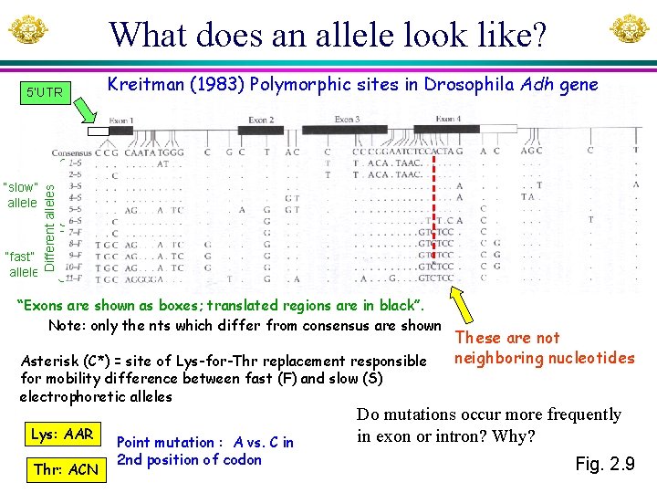
What does an allele look like? “slow” allele “fast” allele Kreitman (1983) Polymorphic sites in Drosophila Adh gene Different alleles 5’UTR “Exons are shown as boxes; translated regions are in black”. Note: only the nts which differ from consensus are shown Asterisk (C*) = site of Lys-for-Thr replacement responsible for mobility difference between fast (F) and slow (S) electrophoretic alleles Lys: AAR Thr: ACN Point mutation : A vs. C in 2 nd position of codon These are not neighboring nucleotides Do mutations occur more frequently in exon or intron? Why? Fig. 2. 9

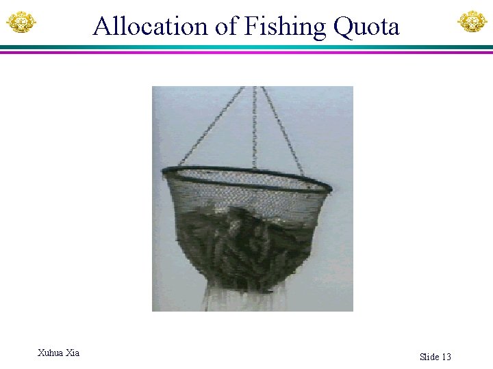
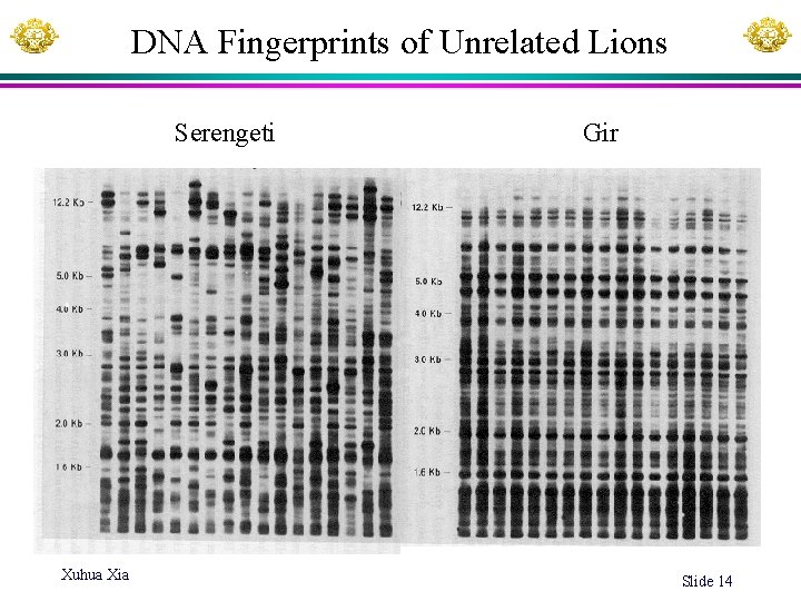
What can we do with alleles? • Mating system and paternity determination • Genetic markers for species identification as a tool of species protection • DNA finger prints for fishing quota allocation • Genetic diversity as an index of population health Xuhua Xia Slide 8

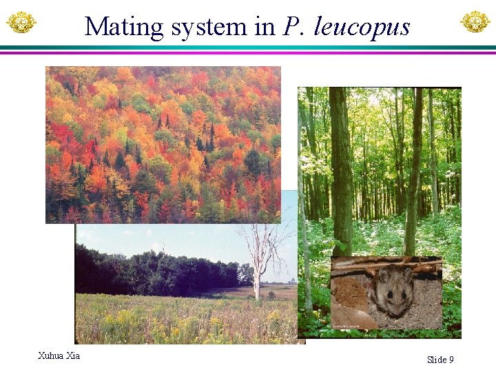
Mating system in P. leucopus Xuhua Xia Slide 9

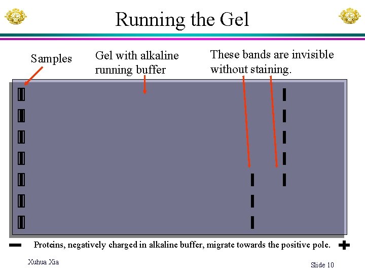
Running the Gel Samples Gel with alkaline running buffer These bands are invisible without staining. Proteins, negatively charged in alkaline buffer, migrate towards the positive pole. Xuhua Xia Slide 10

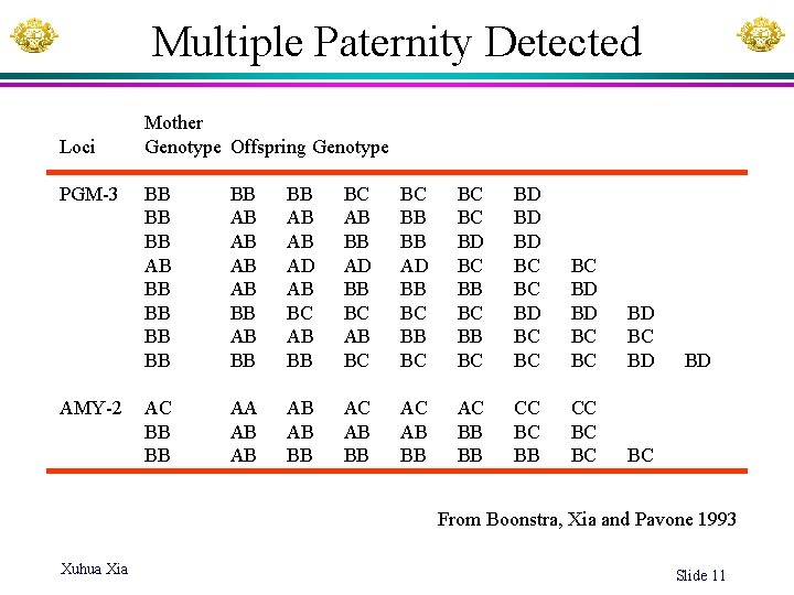
Multiple Paternity Detected Loci PGM-3 AMY-2 Mother Genotype Offspring Genotype BB BB BB AB AB BB BB AB AB AD AB BC AB BB AD BB BC AB BC BC BB BB AD BB BC BC BC BD BC BB BC BD BD BD BC BC BC BD BD BC BC BD AC BB BB AA AB AB BB AC BB BB CC BC BC BC BD From Boonstra, Xia and Pavone 1993 Xuhua Xia Slide 11

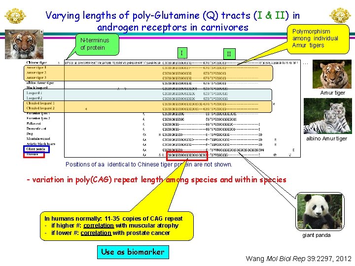
Varying lengths of poly-Glutamine (Q) tracts (I & II) in androgen receptors in carnivores Polymorphism N-terminus of protein among individual Amur tigers I II … Amur tiger albino Amur tiger Positions of aa identical to Chinese tiger protein are not shown. - variation in poly(CAG) repeat length among species and within species In humans normally: 11 -35 copies of CAG repeat - if higher #: correlation with muscular atrophy - if lower #: correlation with prostate cancer Use as biomarker giant panda Wang Mol Biol Rep 39: 2297, 2012

Allocation of Fishing Quota Xuhua Xia Slide 13

DNA Fingerprints of Unrelated Lions Serengeti Xuhua Xia Gir Slide 14

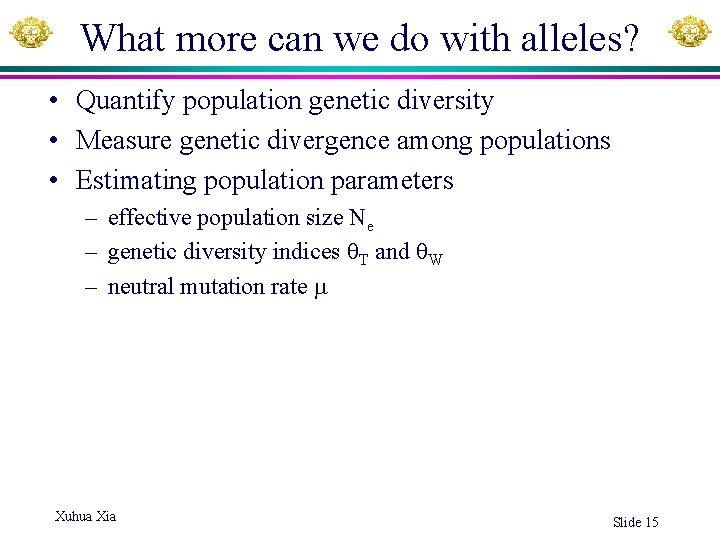
What more can we do with alleles? • Quantify population genetic diversity • Measure genetic divergence among populations • Estimating population parameters – effective population size Ne – genetic diversity indices T and W – neutral mutation rate Xuhua Xia Slide 15

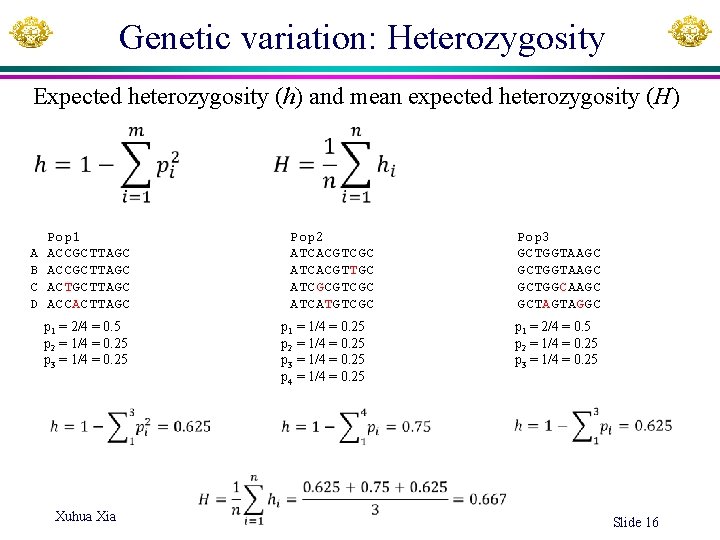
Genetic variation: Heterozygosity Expected heterozygosity (h) and mean expected heterozygosity (H) A B C D Pop 1 ACCGCTTAGC ACTGCTTAGC ACCACTTAGC p 1 = 2/4 = 0. 5 p 2 = 1/4 = 0. 25 p 3 = 1/4 = 0. 25 Xuhua Xia Pop 2 ATCACGTCGC ATCACGTTGC ATCGCGTCGC ATCATGTCGC p 1 = 1/4 = 0. 25 p 2 = 1/4 = 0. 25 p 3 = 1/4 = 0. 25 p 4 = 1/4 = 0. 25 Pop 3 GCTGGTAAGC GCTGGCAAGC GCTAGTAGGC p 1 = 2/4 = 0. 5 p 2 = 1/4 = 0. 25 p 3 = 1/4 = 0. 25 Slide 16

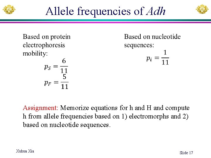
Allele frequencies of Adh Assignment: Memorize equations for h and H and compute h from allele frequencies based on 1) electromorphs and 2) based on nucleotide sequences. Xuhua Xia Slide 17

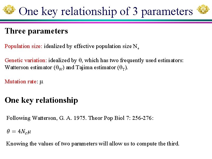
One key relationship of 3 parameters Three parameters Population size: idealized by effective population size Ne Genetic variation: idealized by , which has two frequently used estimators: Watterson estimator ( W) and Tajima estimator ( T). Mutation rate: One key relationship Following Watterson, G. A. 1975. Theor Pop Biol 7: 256 -276: Knowing the values of two parameters will allow us to compute third.

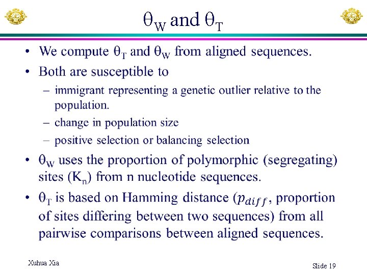
W and T • Xuhua Xia Slide 19

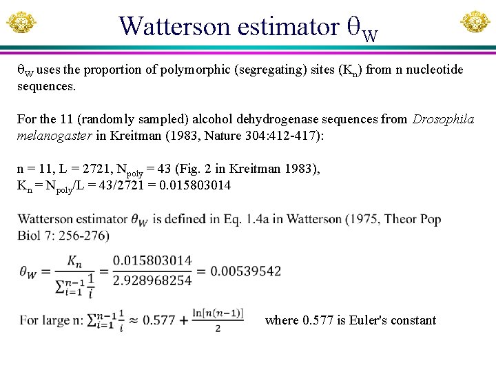
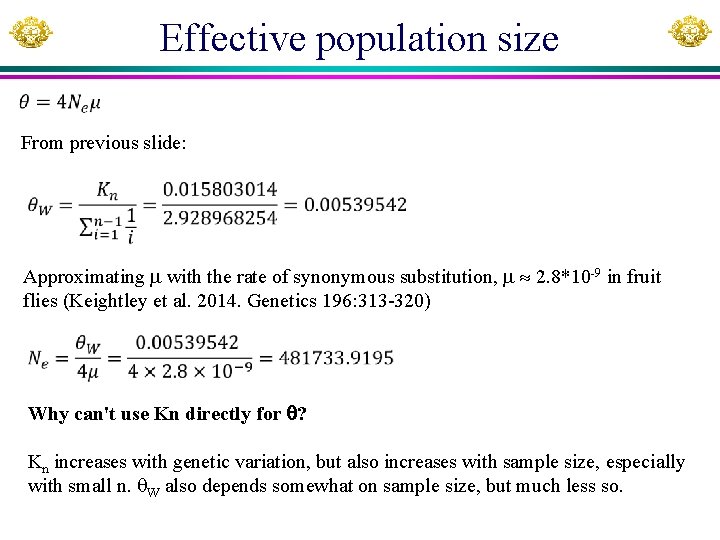
Watterson estimator W W uses the proportion of polymorphic (segregating) sites (Kn) from n nucleotide sequences. For the 11 (randomly sampled) alcohol dehydrogenase sequences from Drosophila melanogaster in Kreitman (1983, Nature 304: 412 -417): n = 11, L = 2721, Npoly = 43 (Fig. 2 in Kreitman 1983), Kn = Npoly/L = 43/2721 = 0. 015803014 where 0. 577 is Euler's constant

Effective population size From previous slide: Approximating with the rate of synonymous substitution, 2. 8*10 -9 in fruit flies (Keightley et al. 2014. Genetics 196: 313 -320) Why can't use Kn directly for ? Kn increases with genetic variation, but also increases with sample size, especially with small n. W also depends somewhat on sample size, but much less so.

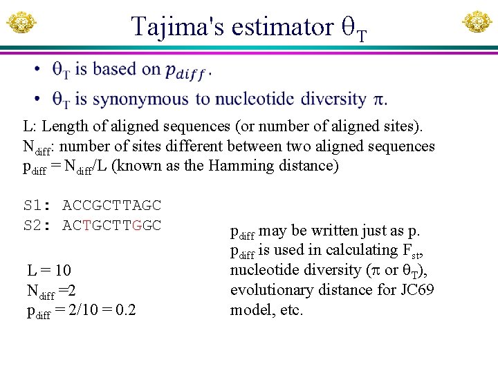
Tajima's estimator T • L: Length of aligned sequences (or number of aligned sites). Ndiff: number of sites different between two aligned sequences pdiff = Ndiff/L (known as the Hamming distance) S 1: ACCGCTTAGC S 2: ACTGCTTGGC L = 10 Ndiff =2 pdiff = 2/10 = 0. 2 pdiff may be written just as p. pdiff is used in calculating Fst, nucleotide diversity ( or T), evolutionary distance for JC 69 model, etc.

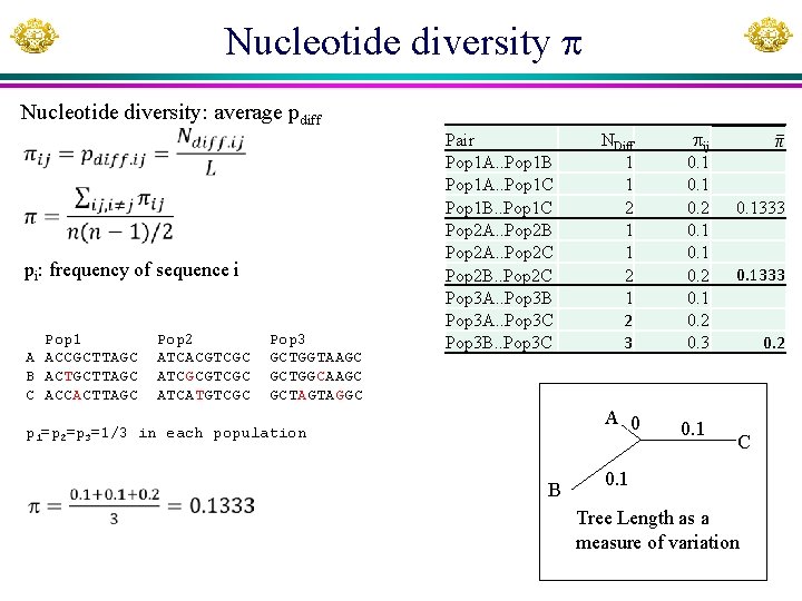
Nucleotide diversity Nucleotide diversity: average pdiff pi: frequency of sequence i Pop 1 A ACCGCTTAGC B ACTGCTTAGC C ACCACTTAGC Pop 2 ATCACGTCGC ATCGCGTCGC ATCATGTCGC Pop 3 GCTGGTAAGC GCTGGCAAGC GCTAGTAGGC Pair Pop 1 A. . Pop 1 B Pop 1 A. . Pop 1 C Pop 1 B. . Pop 1 C Pop 2 A. . Pop 2 B Pop 2 A. . Pop 2 C Pop 2 B. . Pop 2 C Pop 3 A. . Pop 3 B Pop 3 A. . Pop 3 C Pop 3 B. . Pop 3 C NDiff 1 1 2 1 2 3 A 0 p 1=p 2=p 3=1/3 in each population B ij 0. 1 0. 2 0. 3 0. 1333 0. 2 C 0. 1 Tree Length as a measure of variation

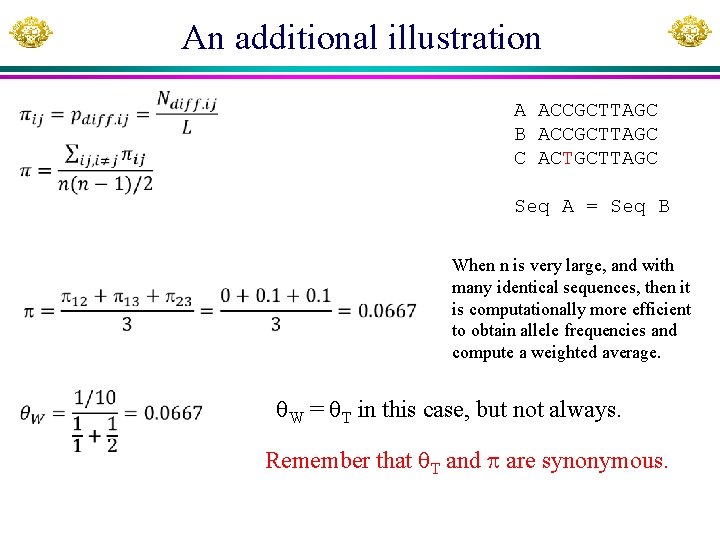
An additional illustration A ACCGCTTAGC B ACCGCTTAGC C ACTGCTTAGC Seq A = Seq B When n is very large, and with many identical sequences, then it is computationally more efficient to obtain allele frequencies and compute a weighted average. W = T in this case, but not always. Remember that T and are synonymous.

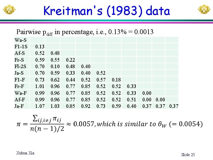
Kreitman's (1983) data Pairwise pdiff in percentage, i. e. , 0. 13% = 0. 0013 Wa-S F 1 -1 S Af-S Fr-S Fl-2 S Ja-S F 1 -F Fr-F Wa-F Af-F Ja-F Xuhua Xia 0. 13 0. 52 0. 59 0. 70 0. 73 1. 01 0. 99 1. 07 0. 48 0. 55 0. 10 0. 59 0. 62 0. 96 1. 03 0. 22 0. 48 0. 33 0. 44 0. 77 0. 85 0. 40 0. 52 0. 85 0. 92 0. 57 0. 52 0. 73 0. 18 0. 52 0. 59 0. 33 0. 51 0. 40 0. 00 0. 37 Slide 25

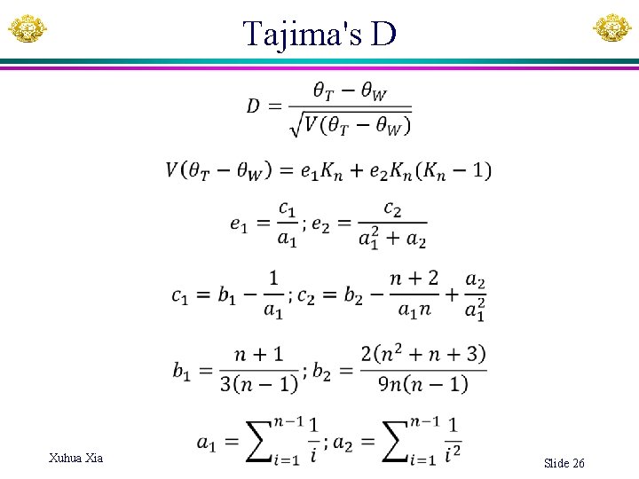
Tajima's D Xuhua Xia Slide 26

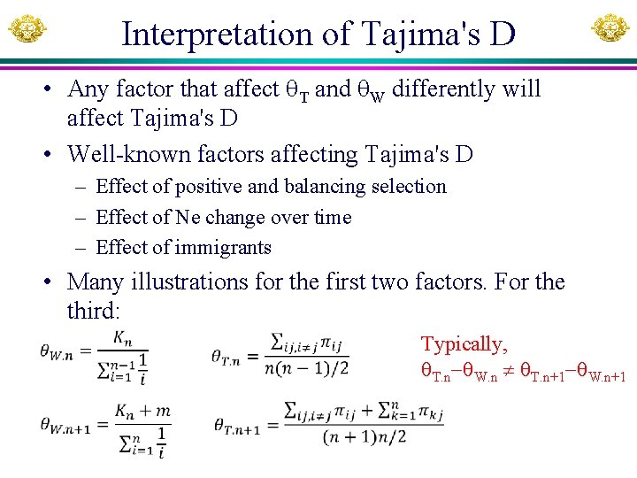
Interpretation of Tajima's D • Any factor that affect T and W differently will affect Tajima's D • Well-known factors affecting Tajima's D – Effect of positive and balancing selection – Effect of Ne change over time – Effect of immigrants • Many illustrations for the first two factors. For the third: Typically, T. n W. n T. n+1 W. n+1

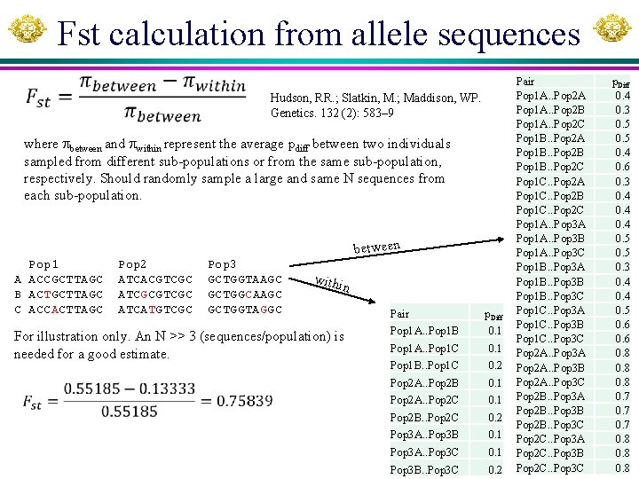
Fst calculation from allele sequences Hudson, RR. ; Slatkin, M. ; Maddison, WP. Genetics. 132 (2): 583– 9 where between and within represent the average pdiff between two individuals sampled from different sub-populations or from the same sub-population, respectively. Should randomly sample a large and same N sequences from each sub-population. between Pop 1 A ACCGCTTAGC B ACTGCTTAGC C ACCACTTAGC Pop 2 ATCACGTCGC ATCGCGTCGC ATCATGTCGC Pop 3 GCTGGTAAGC GCTGGCAAGC GCTGGTAGGC withi n For illustration only. An N >> 3 (sequences/population) is needed for a good estimate. Pair p. Diff Pop 1 A. . Pop 1 B 0. 1 Pop 1 A. . Pop 1 C 0. 1 Pop 1 B. . Pop 1 C 0. 2 Pop 2 A. . Pop 2 B 0. 1 Pop 2 A. . Pop 2 C 0. 1 Pop 2 B. . Pop 2 C 0. 2 Pop 3 A. . Pop 3 B 0. 1 Pop 3 A. . Pop 3 C 0. 1 Pop 3 B. . Pop 3 C 0. 2 Pair Pop 1 A. . Pop 2 A Pop 1 A. . Pop 2 B Pop 1 A. . Pop 2 C Pop 1 B. . Pop 2 A Pop 1 B. . Pop 2 B Pop 1 B. . Pop 2 C Pop 1 C. . Pop 2 A Pop 1 C. . Pop 2 B Pop 1 C. . Pop 2 C Pop 1 A. . Pop 3 A Pop 1 A. . Pop 3 B Pop 1 A. . Pop 3 C Pop 1 B. . Pop 3 A Pop 1 B. . Pop 3 B Pop 1 B. . Pop 3 C Pop 1 C. . Pop 3 A Pop 1 C. . Pop 3 B Pop 1 C. . Pop 3 C Pop 2 A. . Pop 3 A Pop 2 A. . Pop 3 B Pop 2 A. . Pop 3 C Pop 2 B. . Pop 3 A Pop 2 B. . Pop 3 B Pop 2 B. . Pop 3 C Pop 2 C. . Pop 3 A Pop 2 C. . Pop 3 B Pop 2 C. . Pop 3 C p. Diff 0. 4 0. 3 0. 5 0. 4 0. 6 0. 3 0. 4 0. 5 0. 6 0. 8 0. 7 0. 8

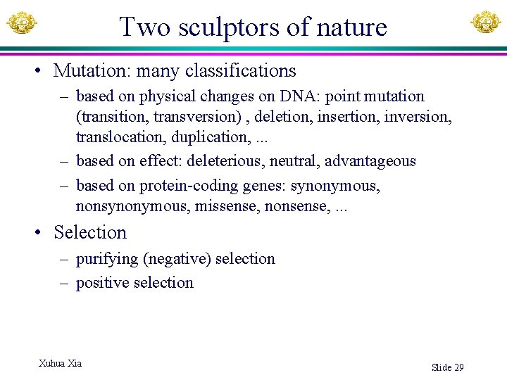
Two sculptors of nature • Mutation: many classifications – based on physical changes on DNA: point mutation (transition, transversion) , deletion, insertion, inversion, translocation, duplication, . . . – based on effect: deleterious, neutral, advantageous – based on protein-coding genes: synonymous, nonsynonymous, missense, nonsense, . . . • Selection – purifying (negative) selection – positive selection Xuhua Xia Slide 29

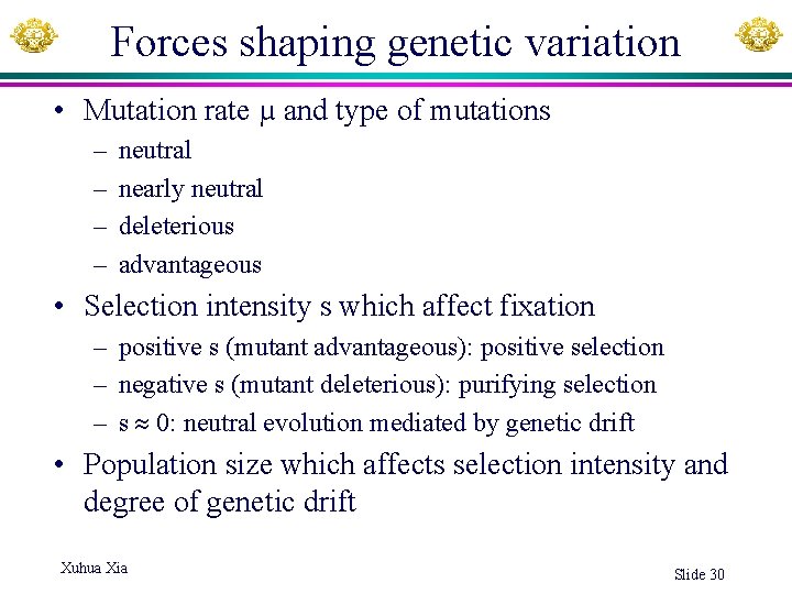
Forces shaping genetic variation • Mutation rate µ and type of mutations – – neutral nearly neutral deleterious advantageous • Selection intensity s which affect fixation – positive s (mutant advantageous): positive selection – negative s (mutant deleterious): purifying selection – s 0: neutral evolution mediated by genetic drift • Population size which affects selection intensity and degree of genetic drift Xuhua Xia Slide 30

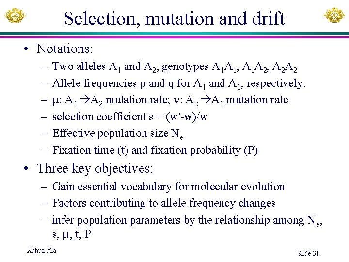
Selection, mutation and drift • Notations: – – – Two alleles A 1 and A 2, genotypes A 1 A 1, A 1 A 2, A 2 A 2 Allele frequencies p and q for A 1 and A 2, respectively. µ: A 1 A 2 mutation rate; : A 2 A 1 mutation rate selection coefficient s = (w'-w)/w Effective population size Ne Fixation time (t) and fixation probability (P) • Three key objectives: – Gain essential vocabulary for molecular evolution – Factors contributing to allele frequency changes – infer population parameters by the relationship among Ne, s, µ, t, P Xuhua Xia Slide 31

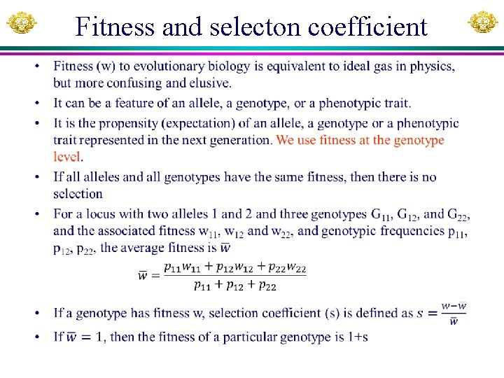
Fitness and selecton coefficient •

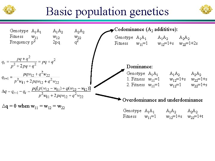
Basic population genetics Genotype A 1 A 1 Fitness w 11 Frequency p 2 A 1 A 2 w 12 2 pq A 2 A 2 w 22 q 2 Codominance (A 2 addititive): Genotype A 1 A 1 Fitness w 11=1 A 1 A 2 w 12=1+s A 2 A 2 w 22=1+2 s Dominance: Genotype A 1 A 1 1. Fitness w 11=1 2. Fitness w 11=1 q = 0 when w 11 = w 12 = w 22 A 1 A 2 w 12=1+s w 12=1 A 2 A 2 w 22=1+s Overdominance and underdominance Genotype A 1 A 1 Fitness w 11=1 A 1 A 2 w 12=1+s A 2 A 2 w 22=1+t

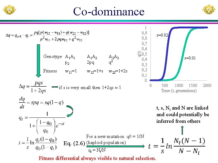
Genotype A 1 A 1 p 2 A 1 A 2 2 pq A 2 A 2 q 2 Fitness w 12=1+s w 22=1+2 s w 11=1 q(t) Co-dominance 1 0, 9 0, 8 0, 7 0, 6 0, 5 0, 4 0, 3 0, 2 0, 1 0 if s is very small then 1+2 qs 1 s=0. 02 s=0. 01 0 500 1000 1500 Time (t, generations) 2000 t, s, Nt and N are linked and could potentially be inferred from others Eq. (2. 6) For a new mutation: q 0 = 1/N (haploid population) qt = Nt/N Fitness differential always visible to natural selection.

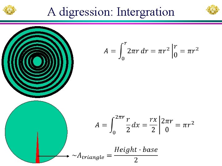
A digression: Intergration

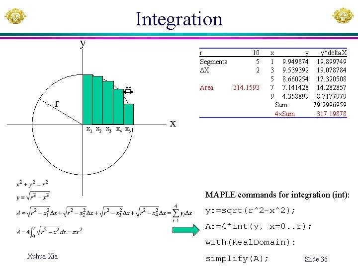
Integration y r Segments X Area x 10 5 2 314. 1593 r x 1 x 2 x 3 x 4 x 5 x x 1 3 5 7 9 y y*delta. X 9. 949874 19. 899749 9. 539392 19. 078784 8. 660254 17. 320508 7. 141428 14. 282857 4. 358899 8. 7177979 Sum 79. 2996959 4 Sum 317. 19878 MAPLE commands for integration (int): y: =sqrt(r^2 -x^2); A: =4*int(y, x=0. . r); with(Real. Domain): Xuhua Xia simplify(A); Slide 36

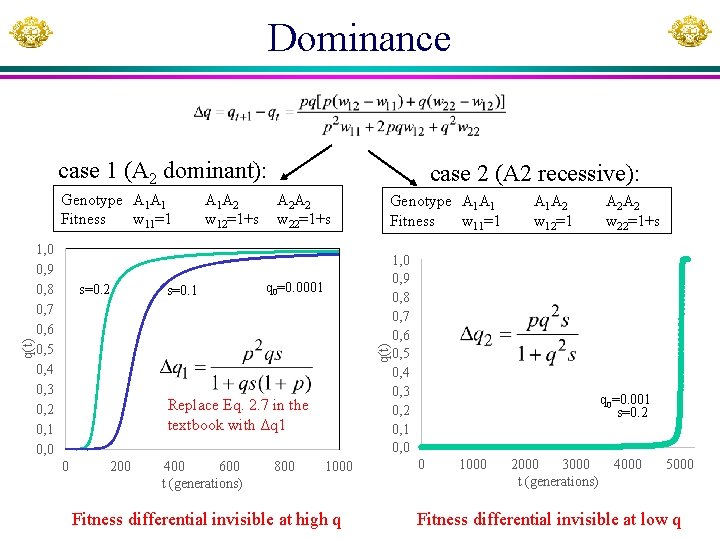
Dominance case 1 (A 2 dominant): 1, 0 0, 9 0, 8 0, 7 0, 6 0, 5 0, 4 0, 3 0, 2 0, 1 0, 0 s=0. 2 A 1 A 2 w 12=1+s s=0. 1 A 2 A 2 w 22=1+s Genotype A 1 A 1 Fitness w 11=1 q 0=0. 0001 q(t) Genotype A 1 A 1 Fitness w 11=1 case 2 (A 2 recessive): Replace Eq. 2. 7 in the textbook with Δq 1 0 200 400 600 t (generations) 800 1000 Fitness differential invisible at high q A 1 A 2 w 12=1 1, 0 0, 9 0, 8 0, 7 0, 6 0, 5 0, 4 0, 3 0, 2 0, 1 0, 0 A 2 A 2 w 22=1+s q 0=0. 001 s=0. 2 0 1000 2000 3000 t (generations) 4000 5000 Fitness differential invisible at low q

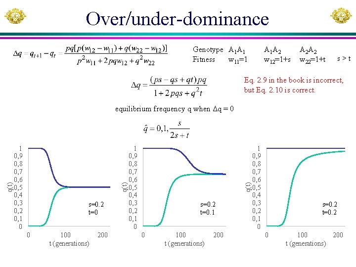
Over/under-dominance Genotype A 1 A 1 Fitness w 11=1 A 1 A 2 w 12=1+s A 2 A 2 w 22=1+t s>t Eq. 2. 9 in the book is incorrect, but Eq. 2. 10 is correct. s=0. 2 t=0 0 100 t (generations) 200 1 0, 9 0, 8 0, 7 0, 6 0, 5 0, 4 0, 3 0, 2 0, 1 0 q(t) equilibrium frequency q when Δq = 0 s=0. 2 t=0. 1 0 100 t (generations) 200 1 0, 9 0, 8 0, 7 0, 6 0, 5 0, 4 0, 3 0, 2 0, 1 0 s=0. 2 t=0. 2 0 100 200 t (generations)

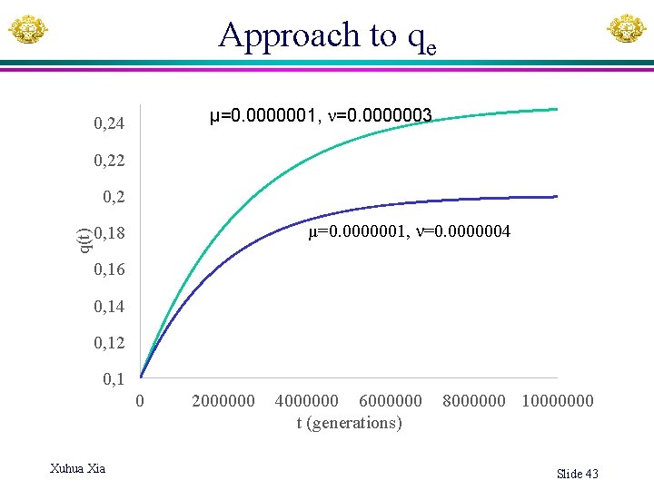
Mutation A locus with two alleles A and B, with frequencies p and q, and µ for mutation rate from A to B and for mutation rate B to A. Xuhua Xia Slide 41

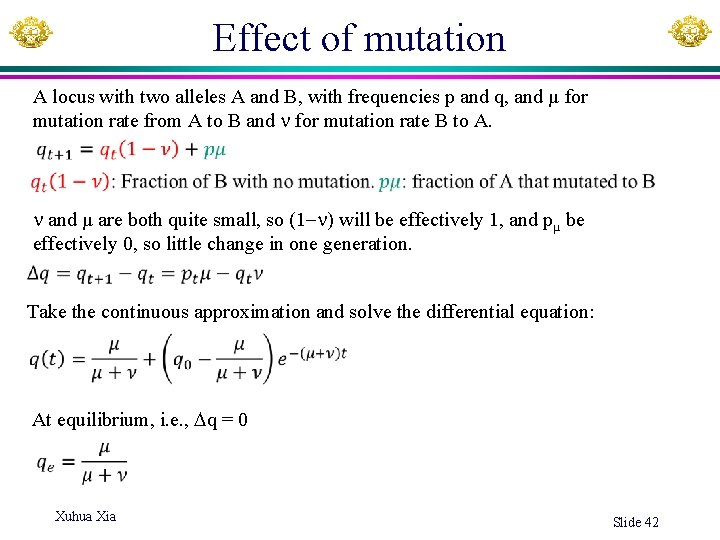
Effect of mutation A locus with two alleles A and B, with frequencies p and q, and µ for mutation rate from A to B and for mutation rate B to A. and µ are both quite small, so (1 ) will be effectively 1, and pµ be effectively 0, so little change in one generation. Take the continuous approximation and solve the differential equation: At equilibrium, i. e. , q = 0 Xuhua Xia Slide 42

Approach to qe µ=0. 0000001, =0. 0000003 0, 24 0, 22 q(t) 0, 2 µ=0. 0000001, =0. 0000004 0, 18 0, 16 0, 14 0, 12 0, 1 0 Xuhua Xia 2000000 4000000 6000000 t (generations) 8000000 10000000 Slide 43

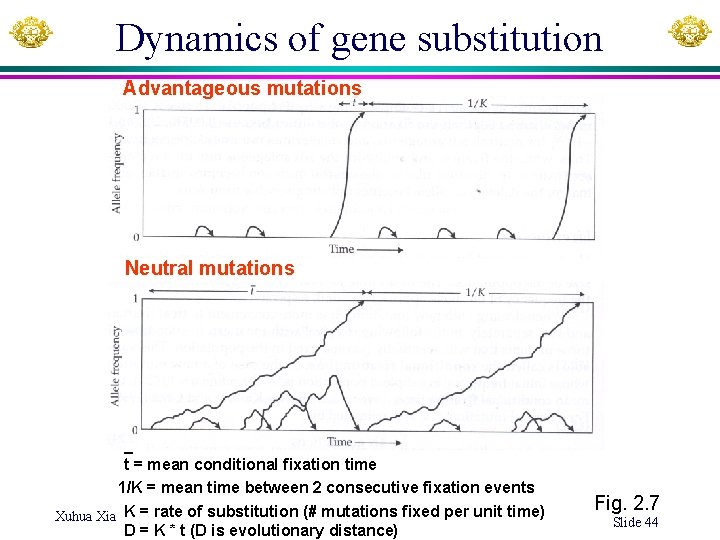
Dynamics of gene substitution Advantageous mutations Neutral mutations _ t = mean conditional fixation time 1/K = mean time between 2 consecutive fixation events Xuhua Xia K = rate of substitution (# mutations fixed per unit time) D = K * t (D is evolutionary distance) Fig. 2. 7 Slide 44

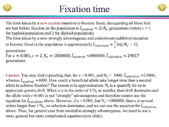
Fixation time

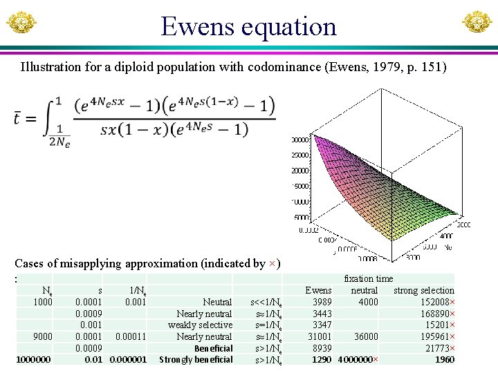
Ewens equation Illustration for a diploid population with codominance (Ewens, 1979, p. 151) Cases of misapplying approximation (indicated by ×) : Ne 1000 9000 1000000 s 1/Ne 0. 0001 0. 0009 0. 001 0. 00011 0. 0009 0. 01 0. 000001 Neutral Nearly neutral weakly selective Nearly neutral Beneficial Strongly beneficial s<<1/Ne s=1/Ne s>1/Ne Ewens 3989 3443 3347 31001 8939 1290 fixation time neutral strong selection 4000 152008× 168890× 15201× 36000 195961× 21773× 4000000× 1960

What can we do with fixation time? • For a nasty bacterial pathogen that resist both antibiotics and phage therapy, can we design a new benign bacterial strain to outcompete it? How long will it take for the new strain to outcompete the pathogen? (The patient would be long dead if fixation time is 1000 years) • Can you think of other application scenario? Xuhua Xia Slide 47

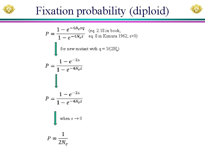
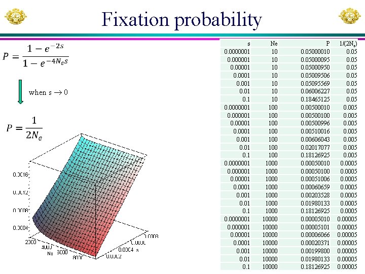
Fixation probability (diploid) (eq. 2. 18 in book, eq. 8 in Kimura 1962, s>0) for new mutant with q = 1/(2 Ne) when s 0

Fixation probability when s 0 s 0. 0000001 0. 00001 0. 001 0. 1 Ne 10 100 100 1000 1000 10000 10000 P 0. 05000010 0. 05000095 0. 05000950 0. 05009506 0. 05095569 0. 06006227 0. 18465125 0. 00500010 0. 00500100 0. 00500996 0. 00510016 0. 00606043 0. 02017077 0. 18126925 0. 00050010 0. 00050100 0. 00051006 0. 00060659 0. 00203528 0. 01980133 0. 18126925 0. 00005010 0. 00005101 0. 00006066 0. 00020371 0. 00199800 0. 01980133 0. 18126925 1/(2 Ne) 0. 05 0. 005 0. 0005 0. 00005 0. 00005

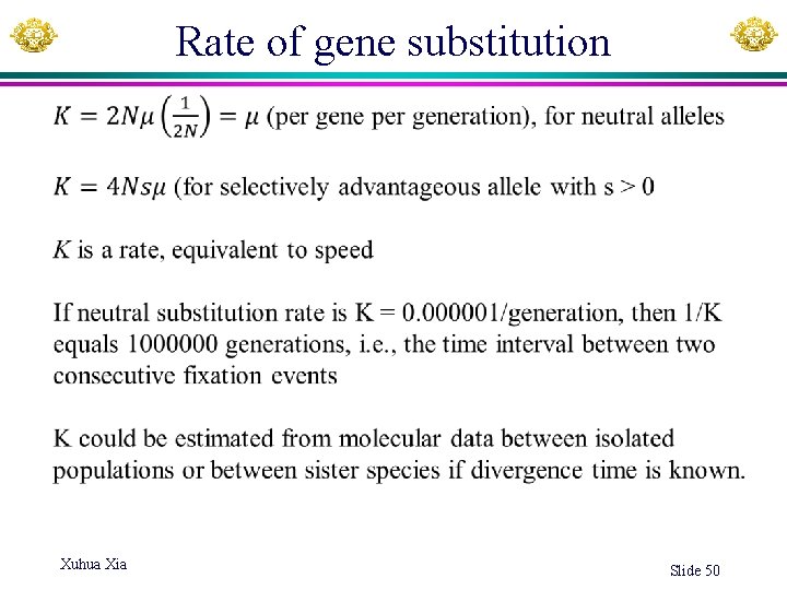
Rate of gene substitution Xuhua Xia Slide 50

Observations leading to Kimura’s theory 1. Relatively high rate of amino acid sequence evolution, especially those of small effect (involving similar amino acids) - variable among proteins, but in many cases about 0. 5 – 1. 5 x 10 -9 changes per non-synonymous (ie. amino acid-altering) site per year (Table 4. 1) 2. Relatively constant rate of evolution for given protein over time - based on pairwise comparisons of proteins (eg a-globin) among species (Figure 4. 15) “Molecular clock” 3. Rate of evolution can differ along protein sequence - functionally important regions (eg active site of enzyme) change at slower rate (Figure 4. 5) 4. High degree of genetic variation (polymorphisms) within populations (Figure 2. 9) Xuhua Xia Slide 51

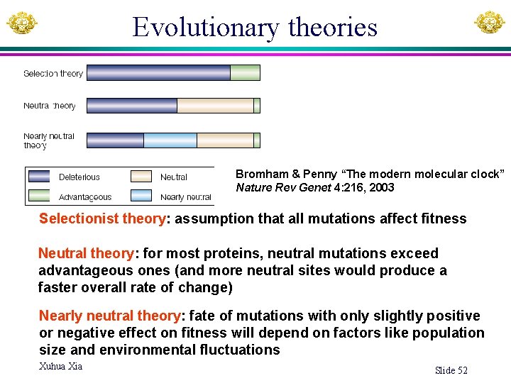
Evolutionary theories Bromham & Penny “The modern molecular clock” Nature Rev Genet 4: 216, 2003 Selectionist theory: assumption that all mutations affect fitness Neutral theory: for most proteins, neutral mutations exceed advantageous ones (and more neutral sites would produce a faster overall rate of change) Nearly neutral theory: fate of mutations with only slightly positive or negative effect on fitness will depend on factors like population size and environmental fluctuations Xuhua Xia Slide 52