Generalized Linear Models Xuhua Xia xxiauottawa ca http

Generalized Linear Models Xuhua Xia xxia@uottawa. ca http: //dambe. bio. uottawa. ca

Ex 1: Spaceship launch • Jan. 28, 1986, the tenth flight of Space Shuttle Challenger (OV-99): failure at 73 seconds into its flight, killing all seven crew members. The spacecraft disintegrated over the Atlantic Ocean, off the coast of Cape Canaveral, Florida, at 11: 39 EST, due to failure of an O-ring seal. • Forecasts for January 28 predicted an unusually cold morning, with temperatures close to − 1 °C (30 °F), the minimum temperature permitted for launch. • Relationship between O-ring failure and temperature Xuhua Xia

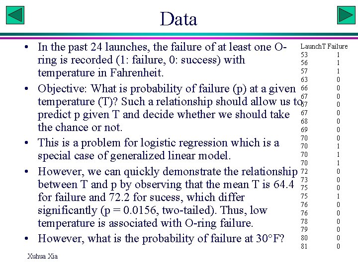
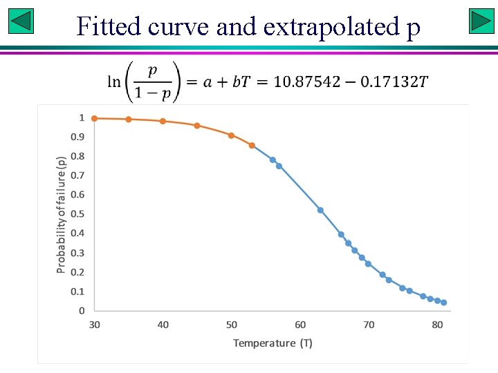
Data Failure • In the past 24 launches, the failure of at least one O- Launch. T 53 1 ring is recorded (1: failure, 0: success) with 56 1 57 1 temperature in Fahrenheit. 63 0 0 • Objective: What is probability of failure (p) at a given 66 67 0 temperature (T)? Such a relationship should allow us to 67 0 0 predict p given T and decide whether we should take 67 68 0 the chance or not. 69 0 70 0 • This is a problem for logistic regression which is a 70 1 special case of generalized linear model. 70 1 0 • However, we can quickly demonstrate the relationship 72 73 0 between T and p by observing that the mean T is 64. 4 75 0 75 1 for failure and 72. 2 for sucess, which differ 76 0 significantly (p = 0. 0156, two-tailed). Thus, low 76 0 78 0 temperature is associated with O-ring failure. 79 0 0 • However, what is the probability of failure at 30°F? 80 81 Xuhua Xia 0

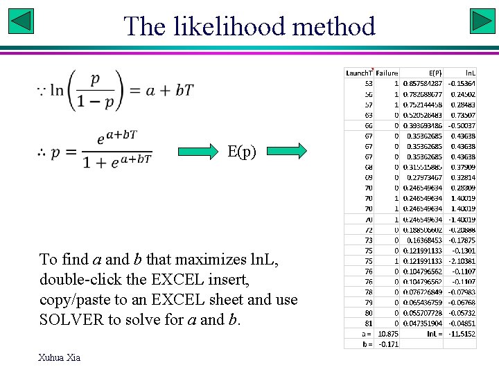
Logistic regression • p: probability of failure • logit: ln(p/q), where q = 1 -p • linear model specifying the relationship between p and T: ln(p/q) = a+b*T, i. e. , p is a function of T with parameters a and b • How to obtain the best estimate of a and b? • There are various approaches to estimate a and b: • The simplest is just to guess: – Failure is less likely in high temperature, i. e. , p decreases with increasing T, so b should be negative. – If T = 0, then p must be close to one (O-rign is not designed to work under such low temperature), so ln(p/q) must be very large, i. e. , a >>0.

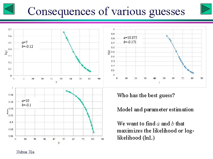
Consequences of various guesses a=7 b=-0. 12 a=10. 875 b=-0. 171 Who has the best guess? a=10 b=-0. 1 Model and parameter estimation We want to find a and b that maximizes the likelihood or loglikelihood (ln. L) Xuhua Xia

The likelihood method E(p) To find a and b that maximizes ln. L, double-click the EXCEL insert, copy/paste to an EXCEL sheet and use SOLVER to solve for a and b. Xuhua Xia

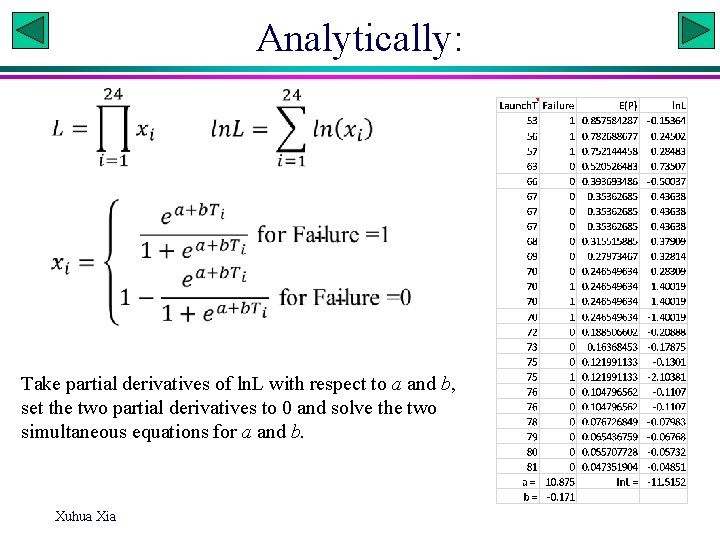
Analytically: Take partial derivatives of ln. L with respect to a and b, set the two partial derivatives to 0 and solve the two simultaneous equations for a and b. Xuhua Xia

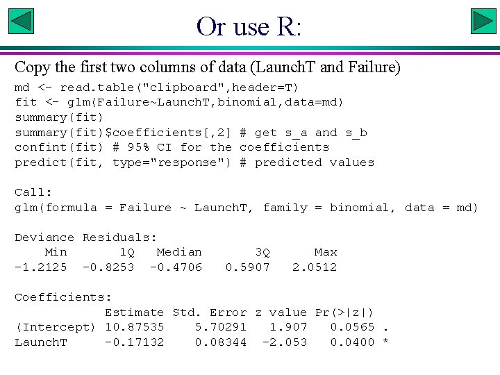
Or use R: Copy the first two columns of data (Launch. T and Failure) md <- read. table("clipboard", header=T) fit <- glm(Failure~Launch. T, binomial, data=md) summary(fit)$coefficients[, 2] # get s_a and s_b confint(fit) # 95% CI for the coefficients predict(fit, type="response") # predicted values Call: glm(formula = Failure ~ Launch. T, family = binomial, data = md) Deviance Residuals: Min 1 Q Median -1. 2125 -0. 8253 -0. 4706 3 Q 0. 5907 Max 2. 0512 Coefficients: Estimate Std. Error z value Pr(>|z|) (Intercept) 10. 87535 5. 70291 1. 907 0. 0565. Launch. T -0. 17132 0. 08344 -2. 053 0. 0400 *

Fitted curve and extrapolated p Xuhua Xia

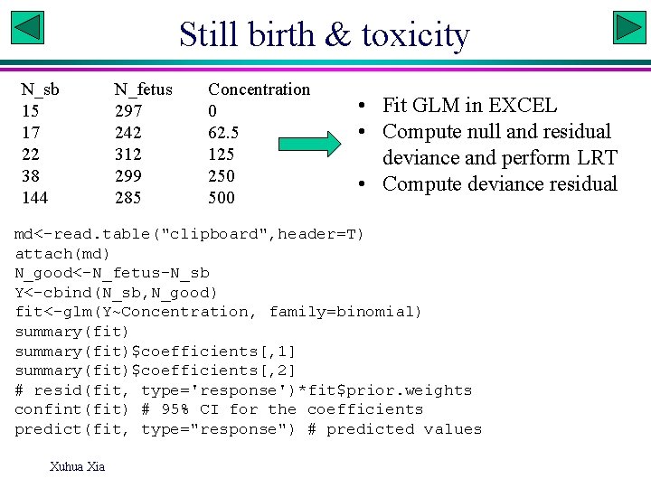
Still birth & toxicity N_sb 15 17 22 38 144 N_fetus 297 242 312 299 285 Concentration 0 62. 5 125 250 500 • Fit GLM in EXCEL • Compute null and residual deviance and perform LRT • Compute deviance residual md<-read. table("clipboard", header=T) attach(md) N_good<-N_fetus-N_sb Y<-cbind(N_sb, N_good) fit<-glm(Y~Concentration, family=binomial) summary(fit)$coefficients[, 1] summary(fit)$coefficients[, 2] # resid(fit, type='response')*fit$prior. weights confint(fit) # 95% CI for the coefficients predict(fit, type="response") # predicted values Xuhua Xia

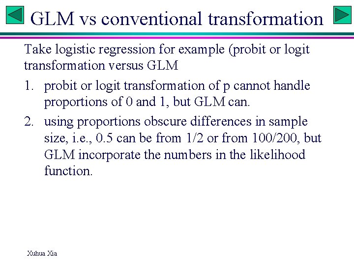
GLM vs conventional transformation Take logistic regression for example (probit or logit transformation versus GLM 1. probit or logit transformation of p cannot handle proportions of 0 and 1, but GLM can. 2. using proportions obscure differences in sample size, i. e. , 0. 5 can be from 1/2 or from 100/200, but GLM incorporate the numbers in the likelihood function. Xuhua Xia

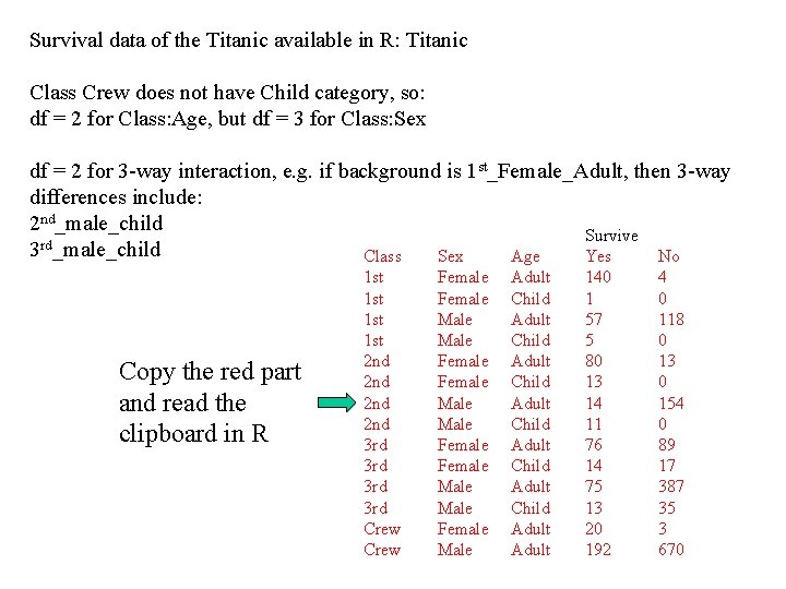
Survival data of the Titanic available in R: Titanic Class Crew does not have Child category, so: df = 2 for Class: Age, but df = 3 for Class: Sex df = 2 for 3 -way interaction, e. g. if background is 1 st_Female_Adult, then 3 -way differences include: 2 nd_male_child Survive 3 rd_male_child Class Sex Age Yes No Copy the red part and read the clipboard in R 1 st 1 st 2 nd 2 nd 3 rd 3 rd Crew Female Male Female Male Adult Child Adult Child Adult 140 1 57 5 80 13 14 11 76 14 75 13 20 192 4 0 118 0 13 0 154 0 89 17 387 35 3 670

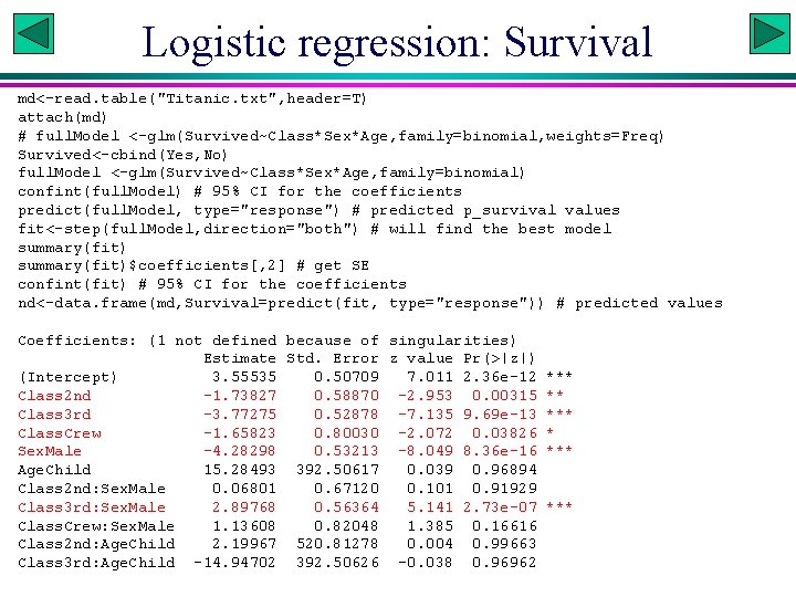
Logistic regression: Survival md<-read. table("Titanic. txt", header=T) attach(md) # full. Model <-glm(Survived~Class*Sex*Age, family=binomial, weights=Freq) Survived<-cbind(Yes, No) full. Model <-glm(Survived~Class*Sex*Age, family=binomial) confint(full. Model) # 95% CI for the coefficients predict(full. Model, type="response") # predicted p_survival values fit<-step(full. Model, direction="both") # will find the best model summary(fit)$coefficients[, 2] # get SE confint(fit) # 95% CI for the coefficients nd<-data. frame(md, Survival=predict(fit, type="response")) # predicted values Coefficients: (1 not defined because of singularities) Estimate Std. Error z value Pr(>|z|) (Intercept) 3. 55535 0. 50709 7. 011 2. 36 e-12 Class 2 nd -1. 73827 0. 58870 -2. 953 0. 00315 Class 3 rd -3. 77275 0. 52878 -7. 135 9. 69 e-13 Class. Crew -1. 65823 0. 80030 -2. 072 0. 03826 Sex. Male -4. 28298 0. 53213 -8. 049 8. 36 e-16 Age. Child 15. 28493 392. 50617 0. 039 0. 96894 Class 2 nd: Sex. Male 0. 06801 0. 67120 0. 101 0. 91929 Class 3 rd: Sex. Male 2. 89768 0. 56364 5. 141 2. 73 e-07 Class. Crew: Sex. Male 1. 13608 0. 82048 1. 385 0. 16616 Class 2 nd: Age. Child 2. 19967 520. 81278 0. 004 0. 99663 Class 3 rd: Age. Child -14. 94702 392. 50626 -0. 038 0. 96962 *** ***

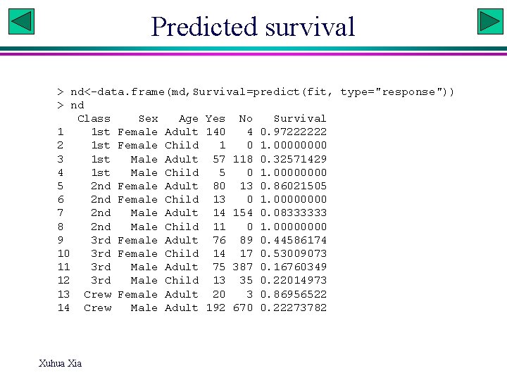
Predicted survival > nd<-data. frame(md, Survival=predict(fit, type="response")) > nd Class Sex Age Yes No Survival 1 1 st Female Adult 140 4 0. 97222222 2 1 st Female Child 1 0 1. 0000 3 1 st Male Adult 57 118 0. 32571429 4 1 st Male Child 5 0 1. 0000 5 2 nd Female Adult 80 13 0. 86021505 6 2 nd Female Child 13 0 1. 0000 7 2 nd Male Adult 14 154 0. 08333333 8 2 nd Male Child 11 0 1. 0000 9 3 rd Female Adult 76 89 0. 44586174 10 3 rd Female Child 14 17 0. 53009073 11 3 rd Male Adult 75 387 0. 16760349 12 3 rd Male Child 13 35 0. 22014973 13 Crew Female Adult 20 3 0. 86956522 14 Crew Male Adult 192 670 0. 22273782 Xuhua Xia