G 205 hydrology First Semester Lesson Two Precipitation

G 205 (hydrology) First Semester Lesson Two

Precipitation

The term precipitation denotes all forms of water that reach the earth from the atmosphere. • • • Rainfall Snowfall Hail Frost dew ﺍﻣﻄﺎﺭ ﺛﻠﻮﺝ ﺣﺎﻟﻮﺏ ﺻﻘﻴﻊ ﻧﺪﻯ

Four conditions must be present for the production of precipitation • • Condensation onto nuclei Colling of the atmosphere Growth of water droplets Mechanics to cause a sufficient density of the droplets

Condensation is the process by which vapor changes to a liquid or solid In the atmosphere, water droplets form on condensation nuclei Sea salts Size of these nuclei < 1 micron Condensation nuclei Combustion products

Prior to precipitation, most water droplets and ice crystals in clouds are < 10 micron ( m) During the condensation process, the water droplet and ice crystals will tend to enlarge because of vapor pressure difference However, without any other factors present, it takes one or more two days for the particles of water and ice to reach the size of a small raindrop (3000 m)

Collision of particles Other factors • Collisions occur because of difference in rising and falling velocities • Particles that collide usually coalesce to form large particles • Gravity acts on the particle to increase the falling velocity, but the friction drag caused a terminal velocity that depends on temperature, pressure, and size of raindrop Crystal growth • When ice elements form a vapor pressure imbalance with the water, larger water drops are created • To rebalance the water vapor evaporates and condense on the ice and thus larger particles are formed

Precipitation Forms Snow is complex ice crystals. The average water content of snow is assumed to be about 10% of an equal volume of water. Hailstones are balls of ice that are about 5 to over 125 mm in diameter. Their specific gravity is about 0. 7 to 0. 9. Thus, hailstones have the potential for agricultural and other property damage

Precipitation Forms Sleet results from the freezing of raindrops and is usually a combination of snow and rain Rain liquid water drops of a size 0. 5 mm to about 7 mm in diameter. Drizzle small water drops less than 0. 5 mm in diameter. The settling velocity is slow, with the intensity rarely exceeding 1 mm/hr (0. 04 in. /hr).

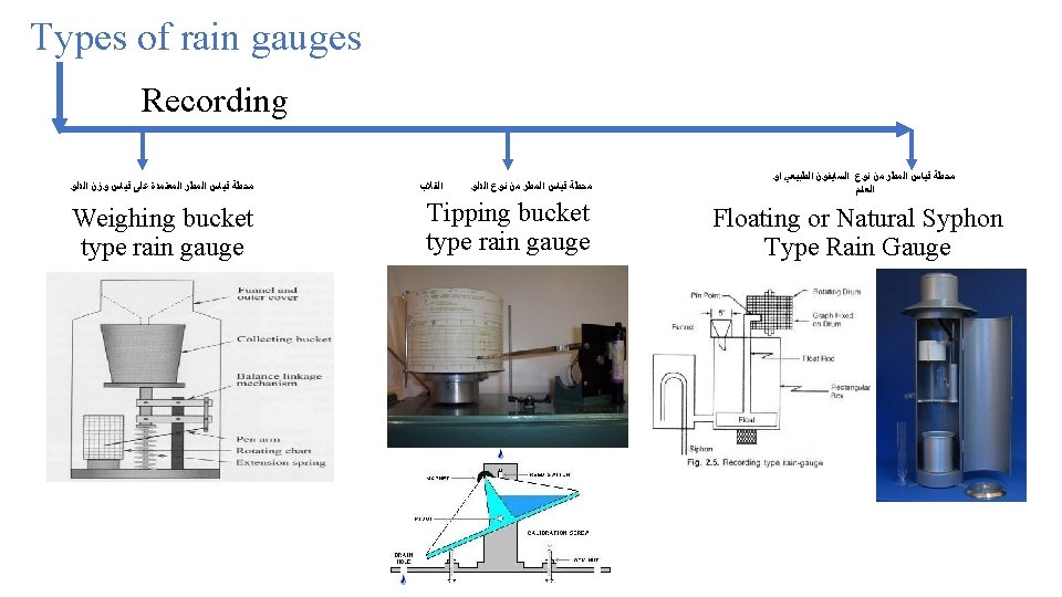
Types of rain gauges Non-recording

Rainy days When the rainfall during a day is 2. 5 mm or more the day is known as rainy day. Classification of intensity of rainfall The rainfall intensity is classified as follows: 1. Up to 2. 5 mm/h : light rain 2. 2. 5 – 7. 5 mm/h : medium rain 3. 7. 5 mm/h and above : heavy rain

Correction of deficiencies in rainfall data Sometimes there might be breaks or gaps in the rainfall data of some stations. These gaps may be due to the following reasons: Absence of an observer Instruments failure Unapproachable circumstances such as flooding

Correction for the missing rainfall data The missing rainfall data may be supplemented by the following method: • Arithmetic average method • Normal ratio method • Weighted average method

Correction for the missing rainfall data Arithmetic average When the data of a rain gauge station, e. g. ‘A’, is missing for a year, consider the adjacent rain gauge stations—B, C and D. If the rainfall at these adjacent stations B, C and D is within 10% of the average rainfall of A (less or more), then the simple arithmetic average of these adjacent stations of the year may be considered as the missing rainfall of A for that year where, n = Number of adjacent rain gauge stations PB, PC, PD = Precipitation at B, C and D for the period for which the data is missing at A

Example 1 In a catchment area, daily precipitation was observed by 11 rain gauge stations. On 2 August 2005, the observations indicated that one rain gauge was out of order. The observations taken by the 10 rain gauge stations are as follows: Estimate the missing data at H. solution

Correction for the missing rainfall data Normal ratio method If the rainfall of station A is missing for a year and the variation of the adjacent rain gauge stations B, C and D is more than 10%, then simple principle of linearity is used to evaluate the missing rainfall of A as follows: where, NA = Average of A excluding the missing period NB NC = Average of B and C excluding the missing period PB PC = Precipitation at B and C during the missing period n = number of adjacent rain gauge stations considered For this method, a minimum of three adjacent rain gauge stations are considered.

Example 2 The average annual precipitation at five rain gauge stations in a catchment is as follows: However, the precipitation at station P was not available for the year 1996 because the rain gauge was out of order. The precipitation observed at the other stations for 1996 was as follows: Evaluate the precipitation at P during 1996. solution

Correction for the missing rainfall data Weighted Average Method The station of which the data is missing, e. g. A, is considered as the origin and the adjacent rain gauge stations are considered and their distances from A are calculated or measured on a map. It is assumed that the rainfall variation between these two stations A and B is inversely proportional to the square of the distance between them. Thus, where, r 1, r 2 and r 3 = the distances from A of the adjacent stations B, C and D PB, PC and PD = the rainfall at the adjacent stations B, C and D for the missing period. This method is also known as United States National Weather Service (USNWS) method.

Example 3 The relative positions of the stations A, B, C and D with respect to X are shown

Example 3 The annual precipitation at X for the year 2005 is missing. The annual precipitation at the remaining four stations for 2005 is as follows: Evaluate the missing precipitation at X for the year 2005. solution The relative positions of the stations A, B, C and D w. r. t. X are : AX = √(202 + 252) = 32. 01 km BX = √(402 + 152) = 42. 72 km CX = √(302 + 202) = 36. 05 km DX = √(252 + 152) = 29. 15 km

Example 3

Consistency verification of rainfall data records It may happen that the rainfall recorded by a rain gauge station is doubtful. It then becomes necessary to verify the rainfall record of this station. This is known as verification of consistency of a rain gauge. This may by due to the following reasons: Change in the location of the rain gauge Change in the surroundings, namely, growth of trees, buildings, and so on. Change in the instrument Fault developed in the rain gauge The verification can be done by the double mass curve method.

Double Mass Curve method On a simple graph paper, the mass curve of the precipitation of the doubtful station, e. g. ‘A’ versus the mass curve of the average precipitation for the remaining rain gauge stations whose data are available for the corresponding period is plotted.

Double Mass Curve method Normally, one should get a straight line through origin if the record at A is correct. If there is inconsistency at A from a particular year, the slope of the straight line may change from that year. It may, therefore, be concluded that the records of A are incorrect from that year and need modification. The slope of the straight line is maintained and extended and the record of A is corrected accordingly. This procedure cannot be applied for studies for storm rainfall or daily rainfall.

Example 4 The average annual precipitation data of six rain gauge stations in a catchment area during 1991– 2000 are as follows: The data observed at station C were doubtful because of some topographical changes there. Verify whether the data observed at C is consistent and correct it, if necessary.

solution The mass curve coordinates of precipitation at C and also the combined mass curve coordinates of precipitation at A, B, D, E and F will be as follows:

solution

Average depth of precipitation The precipitation over a catchment area is never uniform. This becomes quite clear from the figures of the average depth of precipitation of the various rain gauge stations in the catchment area. One of the basic requirements in the study of a catchment area is the average depth of precipitation over the entire catchment. This is also known as equivalent uniform depth of rainfall. The average depth of precipitation can be calculated by the following methods: Arithmetic mean method Thiessen polygon method Isohyetal method

Optimum Number of Rain Gauge Stations • The optimum number of rain gauge station N for a catchment is approximated by the following formula: • Where = allowable error in mean rainfall (%), which is generally taken as 10%. Cv= coefficient of variation of rainfall at m stations (%) which is • Where

• • • m = number of rain gauge stations in the catchment pa = precipitation at a particular station P = average precipitation

Example 5 In a catchment area covering 100 km 2, the average annual precipitation observed at five rain gauge stations is as under. Additional rain gauge stations required = 7 − 5 = 2 Rain gauge density = 100/7 = 14. 30 km 2/rain gauge

Interpretation and quantification of precipitation data • To size water transport and storage systems, quantitative data for rainfall events must be provided. These data can be defined in terms of 1. Intensity (rate of rainfall), usually an average value for a given duration. 2. Duration of storm 3. Time distribution of rainfall over the duration of storm 4. Return period 5. Associated depth of rain

Intensity – duration relationship • The greater the intensity of rainfall, in general the shorter length of time it continues. A formula expressing the connection would be of the type: where i = intensity (mm/h), t = time (h), a and b are locality constants, and for durations greater than two hours where c and n are locality constants

Intensity – duration – frequency relationships • Two important stormwater parameters, intensity and duration, can be statistically related to the frequency of occurrence. The graphical representation of this relationship is the intensity-duration-frequency (IDF) curve. • The IDF curve is a plot of average rainfall intensity versus rainfall duration for various frequency of occurrences ( return period). • This information can also be presented as an isohyetal map of intensity over an area for a given return period and duration. • These data are used for the design and operation of closed or open conduits, reservoirs, groundwater pumps, pollution control structures, . . etc.

Log scale (Rainfall intensity) 50 25 10 5 2 Log scale (duration)

Depth – area – time relationships • Precipitation rarely occurs uniformly over an area. • Holland has shows that ratio between and areal rainfall over area up to 10 km 2 and for storms lasting from 2 To 120 min. is given by Where P = average rain depth over the area P = point rain depth measured at the center of the area A = the area in km 2 t* = an inverse gamma function of storm time obtained from the correlation in figure below

t* Time t (minutes) (logarithm scale)