FITTING HIGH IMPEDANCE DATA ELECTRICAL IMPEDANCE SPECTROSCOPY IS

FITTING HIGH IMPEDANCE DATA • ELECTRICAL IMPEDANCE SPECTROSCOPY IS A POWERFUL TECHNIQUE TO INTERROGATE BARRIER FILMS SUCH AS ORGANIC COATINGS AND OXIDE FILMS. • HOWEVER, THE LARGE DYNAMIC RANGE (6 TO 10 ORDERS OF MAGNITUDE) PRESENT UNIQUE CHALLENGES TO NONLINEAR LEAST SQUARE (NLLS) FIT ENGINES. • CHOICE OF FIT MODEL IS PARAMOUNT TO SUCCESSFUL APPLICATION OF EIS. • THIS PRESENTATION INTRODUCES A FITTING APPLICATION THAT OVERCOMES THESE CHALLENGES. www. eishighimpedanceanalysis. com

THE PEDRA APPLICATION • PEDRA (Parallel Electrical Dielectric Response Analysis) operating under Wave Metrics IGOR PRO offers many advantages over available commercial software. • Pedra is specifically designed to fit high impedance data. • Pedra is efficient, powerful, customizable, flexible and verifiable.

PEDRA IS EFFICIENT • Everything from data import, assigning initial values, fitting convergence tools, displaying both parameters and their associated error (how well a parameter is known), graphical presentation of the fit, residuals between the fit and data and more is done on one screen. • The experimenter can easily interact with the fit routines to “walk” into fit convergence and verify the fit solution.

PEDRA IS POWERFUL • There are resources to: • • • Assign initial values based directly from the imported data Constrain parameters within a certain range Hold and release parameters Exclude data outliers Choice to display circuit parameters or physical attribute parameters Display either capacitor/thickness values or effective capacitor/thickness values; the latter which account for non-ideal behavior

PEDRA IS CUSTOMIZABLE • The program code is open source, written using IGOR PRO’s program language. • The resource tools in IGOR PRO allow program changes on the fly. • The program can be altered, immediately complied and run. • Report graphs can be edited directly on screen to change axis properties, data point and line attributes, introduce multiple axis and much more.

PEDRA IS FLEXIBLE • The number of dielectric responses resemble individual passive highpass filters, the number of which can be added or subtracted to match the complexity of the barrier film. • Parameters can be edited and held during the fit process. • Parameter constraints, effective dielectric constants, surface area, number of fit iterations, error alarm thresholds, use or release constraints can be changed as necessary during the fit.

PEDRA IS VERIFIABLE • The believability of the fit can be assessed by directly observing data point fit/line overlay, parametric and experimental error, fit residuals and ability to switch between circuit and physical display of parameters. • Physical attributes determined using PEDRA has been independently verified: • Thickness determined from EIS has been compared to independent measurements using Optical Microscopy, SEM, TEM, Eddy Current and FTIR (Fast Fourier Transform Infrared Reflective Spectroscopy (FTIR). • • Ionic Resistance paths penetrating the barrier film have been observed using TEM Power law term, n, has been correlated fractional (fractal) properties using surface AFM

PEDRA – UNIQUE FIT MODEL • PEDRA is unique by the fact that the fitting model is based on how the instrument “sees” the data as a function of applied frequency and impedance response. • This is in contrast to the more popular models, where either the empirical or physical model is based on the perception of the experimenter. • The latter perception based models significantly contribute to the amount of disagreement in interpretation between researchers and weaken the application of the technique.

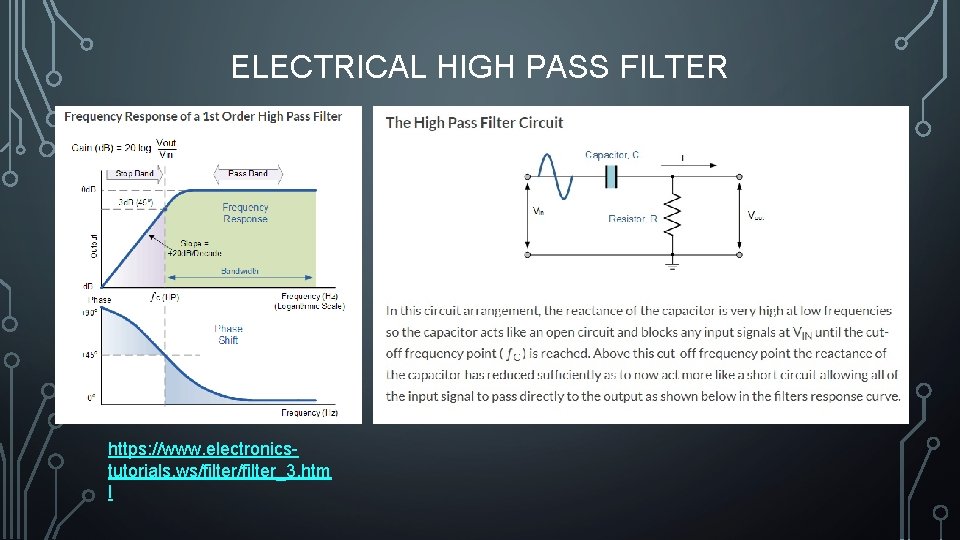
MODEL – PARALLEL COMBINATION OF PASSIVE HIGH-PASS FILTERS • The EIS instrument measures the AC current response as a function of frequency. • AC current can pass through the barrier by independent current paths associated with the barrier film. • Each path has a unique cut-off frequency (time constant) • Above the cut-off frequency current is limited by the series ionic resistance. • Below the cut-off frequency current is limited by the film capacitance.

ELECTRICAL HIGH PASS FILTER https: //www. electronicstutorials. ws/filter_3. htm l

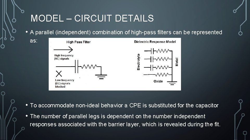
MODEL – CIRCUIT DETAILS • A parallel (independent) combination of high-pass filters can be represented as: • To accommodate non-ideal behavior a CPE is substituted for the capacitor • The number of parallel legs is dependent on the number independent responses associated with the barrier layer, which is revealed during the fit.

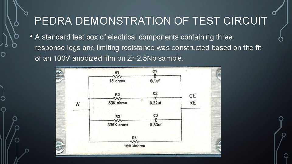
PEDRA DEMONSTRATION OF TEST CIRCUIT • A standard test box of electrical components containing three response legs and limiting resistance was constructed based on the fit of an 100 V anodized film on Zr-2. 5 Nb sample.

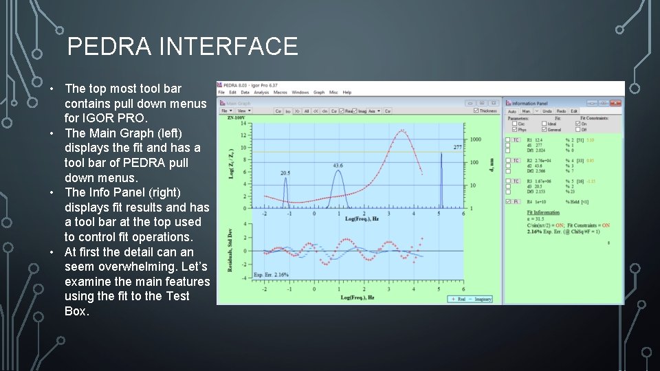
PEDRA INTERFACE • The top most tool bar contains pull down menus for IGOR PRO. • The Main Graph (left) displays the fit and has a tool bar of PEDRA pull down menus. • The Info Panel (right) displays fit results and has a tool bar at the top used to control fit operations. • At first the detail can an seem overwhelming. Let’s examine the main features using the fit to the Test Box.

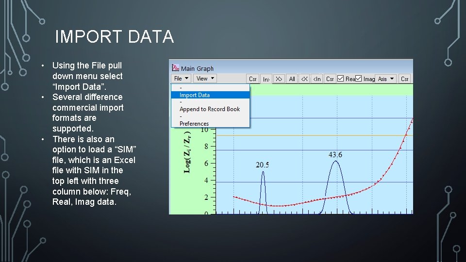
IMPORT DATA • Using the File pull down menu select “Import Data”. • Several difference commercial import formats are supported. • There is also an option to load a “SIM” file, which is an Excel file with SIM in the top left with three column below: Freq, Real, Imag data.

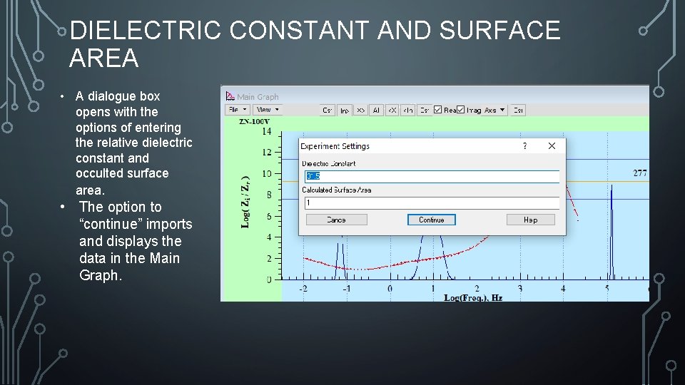
DIELECTRIC CONSTANT AND SURFACE AREA • A dialogue box opens with the options of entering the relative dielectric constant and occulted surface area. • The option to “continue” imports and displays the data in the Main Graph.

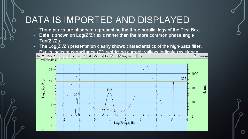
DATA IS IMPORTED AND DISPLAYED • Three peaks are observed representing the three parallel legs of the Test Box. • Data is shown on Log(Z”Z’) axis rather than the more common phase angle Tan(Z”/Z’). • The Log(Z”/Z’) presentation clearly shows characteristics of the high-pass filter. Peaks indicate capacitance (Z”) restricting current; valleys indicate resistance passing current.

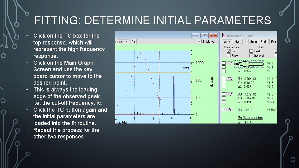
FITTING: DETERMINE INITIAL PARAMETERS • Click on the TC box for the top response, which will represent the high frequency response. • Click on the Main Graph Screen and use the key board cursor to move to the desired point. • This is always the leading edge of the observed peak, i. e. the cut-off frequency, fc. • Click the TC button again and the initial parameters are loaded into the fit routine. • Repeat the process for the other two responses

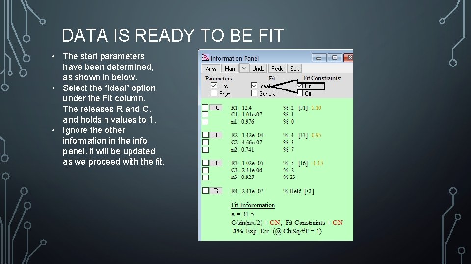
DATA IS READY TO BE FIT • The start parameters have been determined, as shown in below. • Select the “ideal” option under the Fit column. The releases R and C, and holds n values to 1. • Ignore the other information in the info panel, it will be updated as we proceed with the fit.

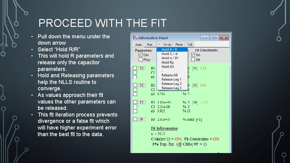
PROCEED WITH THE FIT • Pull down the menu under the down arrow • Select “Hold R/R” • This will hold R parameters and release only the capacitor parameters. • Hold and Releasing parameters help the NLLS routine to converge. • As values approach their fit values the other parameters can be released. • This fit iteration process prevents divergence or a false fit which will have higher experiment error than the best fit to the data.

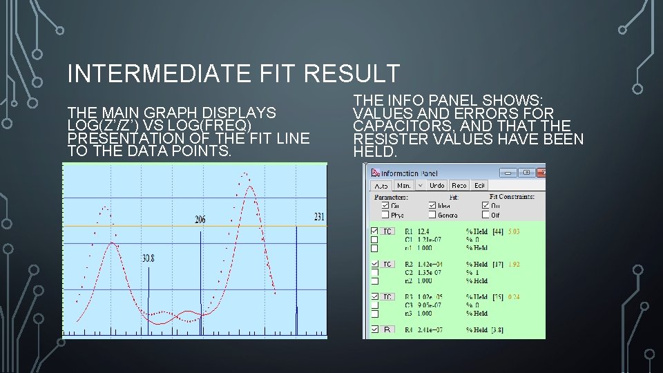
INTERMEDIATE FIT RESULT THE MAIN GRAPH DISPLAYS LOG(Z’/Z’) VS LOG(FREQ) PRESENTATION OF THE FIT LINE TO THE DATA POINTS. THE INFO PANEL SHOWS: VALUES AND ERRORS FOR CAPACITORS, AND THAT THE RESISTER VALUES HAVE BEEN HELD.

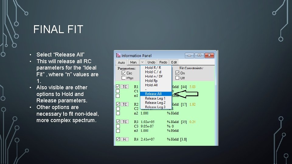
FINAL FIT • Select “Release All” • This will release all RC parameters for the “Ideal Fit” , where “n” values are 1. • Also visible are other options to Hold and Release parameters. • Other options are necessary to fit non-ideal, more complex spectrum.

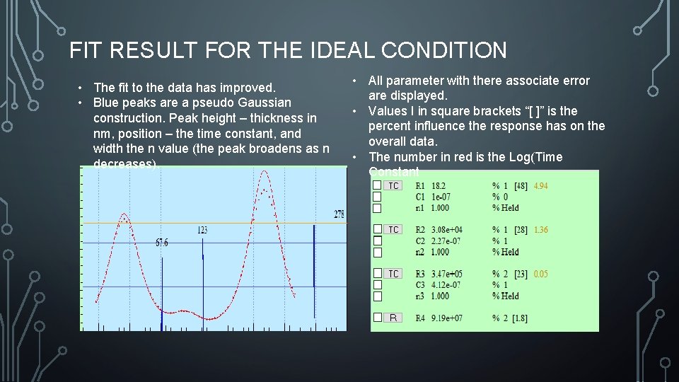
FIT RESULT FOR THE IDEAL CONDITION • The fit to the data has improved. • Blue peaks are a pseudo Gaussian construction. Peak height – thickness in nm, position – the time constant, and width the n value (the peak broadens as n decreases). • All parameter with there associate error are displayed. • Values I in square brackets “[ ]” is the percent influence the response has on the overall data. • The number in red is the Log(Time Constant

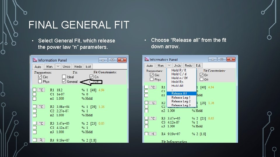
FINAL GENERAL FIT • Select General Fit, which release the power law “n” parameters. • Choose “Release all” from the fit down arrow.

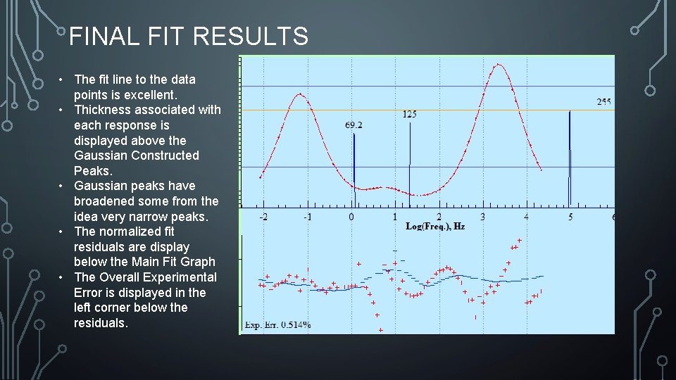
FINAL FIT RESULTS • The fit line to the data points is excellent. • Thickness associated with each response is displayed above the Gaussian Constructed Peaks. • Gaussian peaks have broadened some from the idea very narrow peaks. • The normalized fit residuals are display below the Main Fit Graph • The Overall Experimental Error is displayed in the left corner below the residuals.

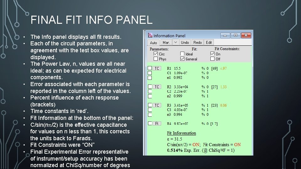
FINAL FIT INFO PANEL • The Info panel displays all fit results. • Each of the circuit parameters, in agreement with the test box values, are displayed. • The Power Law, n, values are all near ideal; as can be expected for electrical components. • Error associated with each parameter is reported in the column left of the values. • Percent influence of each response (brackets) • Time constants in ‘red’. • Fit Information at the bottom of the panel: • C/sin(np/2) is the effective capacitance for values on n less than 1, this corrects the units back to Farads. • Fit Constraints were “ON” • Final Experimental Error representative of instrument/setup accuracy has been normalized at Chi. Sq/number of degrees

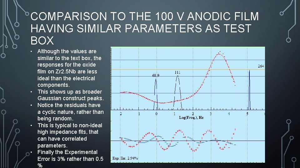
COMPARISON TO THE 100 V ANODIC FILM HAVING SIMILAR PARAMETERS AS TEST BOX • Although the values are similar to the text box, the responses for the oxide film on Zr 2. 5 Nb are less ideal than the electrical components. • This shows up as broader Gaussian construct peaks. • Notice the residuals have a cyclic nature, rather than being random. • This is typical to non-ideal high impedance fits, that can have correlated parameters. • Finally the Experimental Error is 3% rather than 0. 5 %

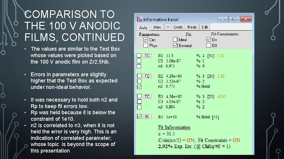
COMPARISON TO THE 100 V ANODIC FILMS, CONTINUED • The values are similar to the Test Box whose values were picked based on the 100 V anodic film on Zr 2. 5 Nb. • Errors in parameters are slightly higher that the Test Box as expected under non-ideal behavior. • It was necessary to hold both n 2 and Rp to keep fit errors low. • Rp was held because it is below the constraint of 1 e 10. • n 2 is correlated to n 3, when it is not held the error is very high. This is an indication of correlated parameter; whose topic is beyond the scope of this presentation

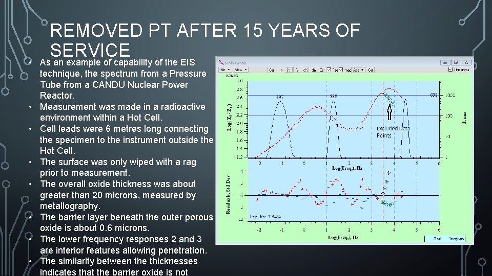
• • REMOVED PT AFTER 15 YEARS OF SERVICE As an example of capability of the EIS technique, the spectrum from a Pressure Tube from a CANDU Nuclear Power Reactor. Measurement was made in a radioactive environment within a Hot Cell leads were 6 metres long connecting the specimen to the instrument outside the Hot Cell. The surface was only wiped with a rag prior to measurement. The overall oxide thickness was about greater than 20 microns, measured by metallography. The barrier layer beneath the outer porous oxide is about 0. 6 microns. The lower frequency responses 2 and 3 are interior features allowing penetration. The similarity between the thicknesses indicates that the barrier oxide is not

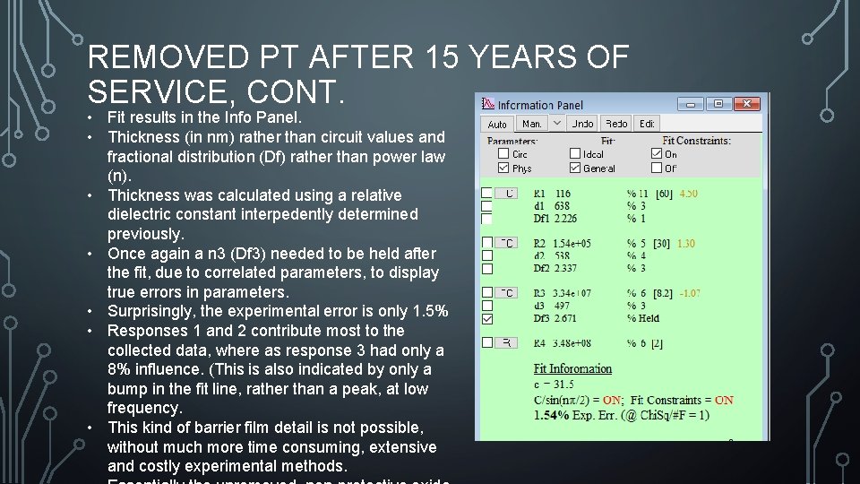
REMOVED PT AFTER 15 YEARS OF SERVICE, CONT. • Fit results in the Info Panel. • Thickness (in nm) rather than circuit values and fractional distribution (Df) rather than power law (n). • Thickness was calculated using a relative dielectric constant interpedently determined previously. • Once again a n 3 (Df 3) needed to be held after the fit, due to correlated parameters, to display true errors in parameters. • Surprisingly, the experimental error is only 1. 5% • Responses 1 and 2 contribute most to the collected data, where as response 3 had only a 8% influence. (This is also indicated by only a bump in the fit line, rather than a peak, at low frequency. • This kind of barrier film detail is not possible, without much more time consuming, extensive and costly experimental methods.

FINAL COMMENTS • THIS PRESENTATION DEMONSTRATES THE POWER, VERSATILITY AND CAPABILITY OF BOTH THE EIS TECHNIQUE AND THE PEDRA ANALYSIS APPLICATION. • THE HIGH PASS FILTER CIRCUIT IS BOTH CAPABLE AND APPROPRIATE TO FIT HIGH IMPEDANCE DIELECTRIC DATA ASSOCIATED WITH COATINGS AND OXIDES. • PEDRA PROVIDES THE EXPERIMENTER WITH AN EFFICIENT, POWERFUL, CUSTOMIZABLE, FLEXIBLE AND VERIFIABLE TOOL TO ANALYZE HIGH IMPEDANCE DATA. • THIS CAPABILITY HAS BEEN DEMONSTRATED FOR: • • • Near-ideal electrical circuits components Well controlled laboratory measurements on anodized films Remote measurement in a harsh environment, with little surface preparation, and after long exposure in an commercial application. • • CONCLUSIONS: • PEDRA IS CAPABLE OF MEETING THE CHALLENGES IN FITTING HIGH IMPEDANCE DATA. THE EIS TECHNIQUE DELIVERS DETAILS OF BARRIER FILM, NOT POSSIBLE WITH OTHER TECHNIQUES. www. eishighimpedanceanalysis. com