False Discovery Rate Guy Yehuda 1 Outline 2

False Discovery Rate Guy Yehuda 1

Outline • • • 2 Short introduction to statistics The problem of multiplicity FDR vs. FWE FDR control procedures and resampling Results of using FDR control procedures Discussion

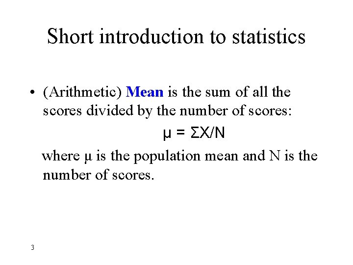
Short introduction to statistics • (Arithmetic) Mean is the sum of all the scores divided by the number of scores: μ = ΣX/N where μ is the population mean and N is the number of scores. 3

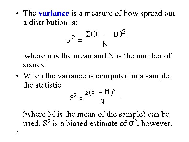
• The variance is a measure of how spread out a distribution is: where μ is the mean and N is the number of scores. • When the variance is computed in a sample, the statistic (where M is the mean of the sample) can be used. S 2 is a biased estimate of σ2, however. 4

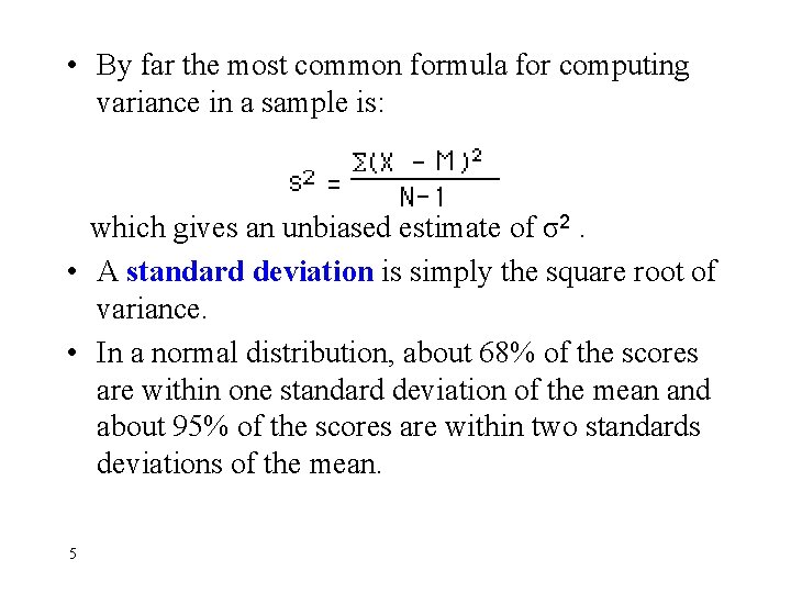
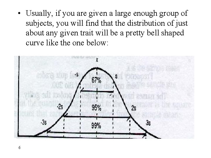
• By far the most common formula for computing variance in a sample is: which gives an unbiased estimate of σ2. • A standard deviation is simply the square root of variance. • In a normal distribution, about 68% of the scores are within one standard deviation of the mean and about 95% of the scores are within two standards deviations of the mean. 5

• Usually, if you are given a large enough group of subjects, you will find that the distribution of just about any given trait will be a pretty bell shaped curve like the one below: 6

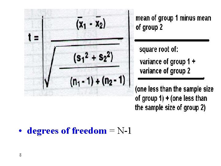
T test A T-test is used to evaluate the statistical similarity of two samples • Gather your data. • Calculate mean and then variance. • Calculate T-statistic. 7

• degrees of freedom = N-1 8

• Null hypothesis (H 0) states that the two samples are identical. • Alternative hypothesis (H 1) states that the samples are statistically different. • A result is significant if it is unlikely to have occurred by chance. • The significance level of a test is the maximum probability of accidentally rejecting a true null hypothesis (a decision known as a Type I Error). The significance of a result is also called its p-value. 9

• We use the degrees of freedom and the t-test in-order to find the p-value in t-statistics table. • If p-value is 0. 03 and the significance level is 0. 05, than the result is significant, i. e. the null hypothesis is rejected. • The power of a statistical test is the probability that the test will reject a false null hypothesis. The higher the power, the greater the chance of obtaining a statistically significant result when the null hypothesis is false. 10

…Back to Microarray World 11

Identifying Differentially Expressed Genes • Individual Hypotheses Testing For each gene use a significance test of 0. 05 level H 0: Gene is similarly expressed H 1: Gene is differently expressed A t-statistic is calculated for comparing gene expression mean between the control and treatment groups. 12

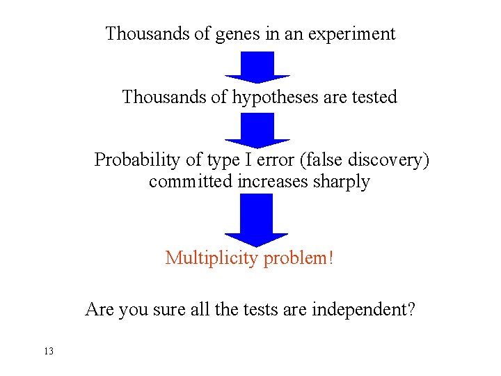
Thousands of genes in an experiment Thousands of hypotheses are tested Probability of type I error (false discovery) committed increases sharply Multiplicity problem! Are you sure all the tests are independent? 13

Are you sure all the tests are independent? • Genes tend to subgroup into highly correlated expression levels for reasons such as co-regulation. • Gene expression measurement errors may be dependent due to factors related to the RNA source, the normalization process etc. We need to account for the dependency structure between the test statistics 14

What shall we do? Let’s pretend there is no (multiplicity) problem! If we deal with 10, 000 genes for example, working at the individual 0. 05 level, would identify, on the average, 10, 000*0. 05=500 differentially expressed genes, even if really no such gene exists! Do we have an extra time and money to waste exploring that amount of genes in vain at later stages? 15

What shall we do? Let’s panic!!! Control the probability of making even one error (or more) - the Family. Wise (type I) Error-rate (FWE) ü The Westfall and Young step-down alg. (WY, 89) ü Holm procedure (79) ü Bonferroni procedure – most conservative Aren’t we missing many genes we need to explore more carefully later ? 16

Is there an in-between approach? Don’t worry, everything is under (FDR) control! 17

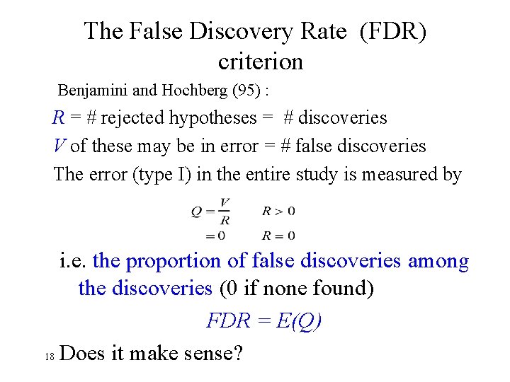
The False Discovery Rate (FDR) criterion Benjamini and Hochberg (95) : R = # rejected hypotheses = # discoveries V of these may be in error = # false discoveries The error (type I) in the entire study is measured by i. e. the proportion of false discoveries among the discoveries (0 if none found) FDR = E(Q) 18 Does it make sense?

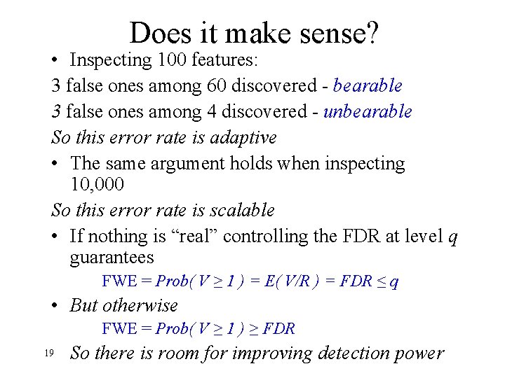
Does it make sense? • Inspecting 100 features: 3 false ones among 60 discovered - bearable 3 false ones among 4 discovered - unbearable So this error rate is adaptive • The same argument holds when inspecting 10, 000 So this error rate is scalable • If nothing is “real” controlling the FDR at level q guarantees FWE = Prob( V ≥ 1 ) = E( V/R ) = FDR ≤ q • But otherwise FWE = Prob( V ≥ 1 ) ≥ FDR 19 So there is room for improving detection power

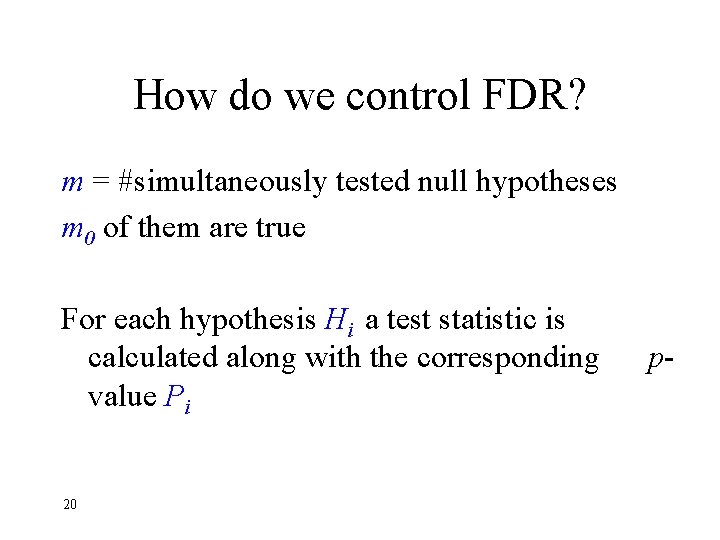
How do we control FDR? m = #simultaneously tested null hypotheses m 0 of them are true For each hypothesis Hi a test statistic is calculated along with the corresponding value Pi 20 p-

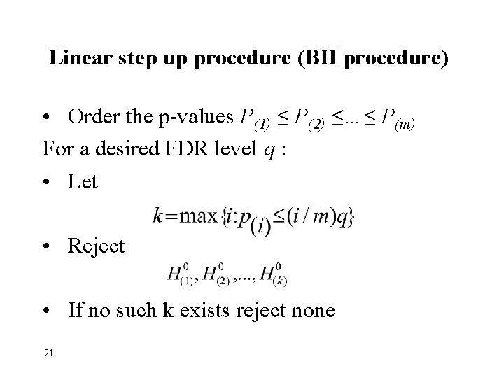
Linear step up procedure (BH procedure) • Order the p-values P(1) ≤ P(2) ≤…≤ P(m) For a desired FDR level q : • Let • Reject • If no such k exists reject none 21

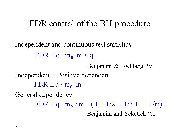
FDR control of the BH procedure Independent and continuous test statistics FDR q · m 0 /m q Benjamini & Hochberg `95 Independent + Positive dependent FDR q · m 0 /m General dependency FDR q · m 0 / m · ( 1 + 1/2 + 1/3 + … 1/m) Benjamini and Yekutieli `01 22

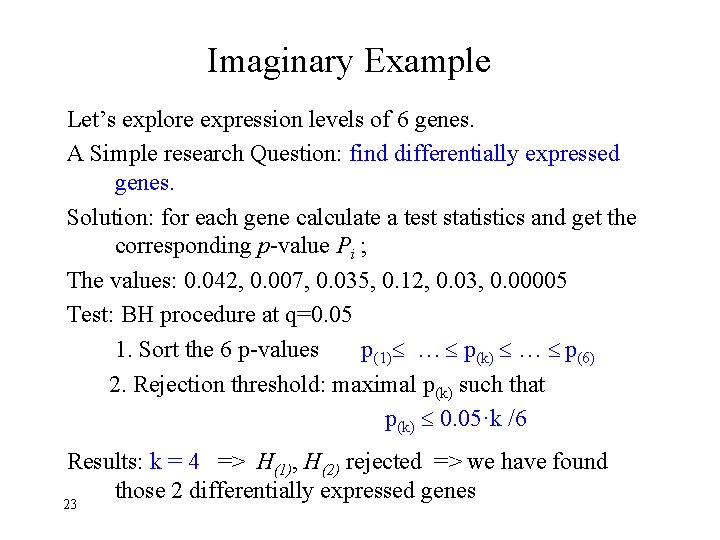
Imaginary Example Let’s explore expression levels of 6 genes. A Simple research Question: find differentially expressed genes. Solution: for each gene calculate a test statistics and get the corresponding p-value Pi ; The values: 0. 042, 0. 007, 0. 035, 0. 12, 0. 03, 0. 00005 Test: BH procedure at q=0. 05 1. Sort the 6 p-values p(1) … p(k) … p(6) 2. Rejection threshold: maximal p(k) such that p(k) 0. 05·k /6 Results: k = 4 => H(1), H(2) rejected => we have found those 2 differentially expressed genes 23

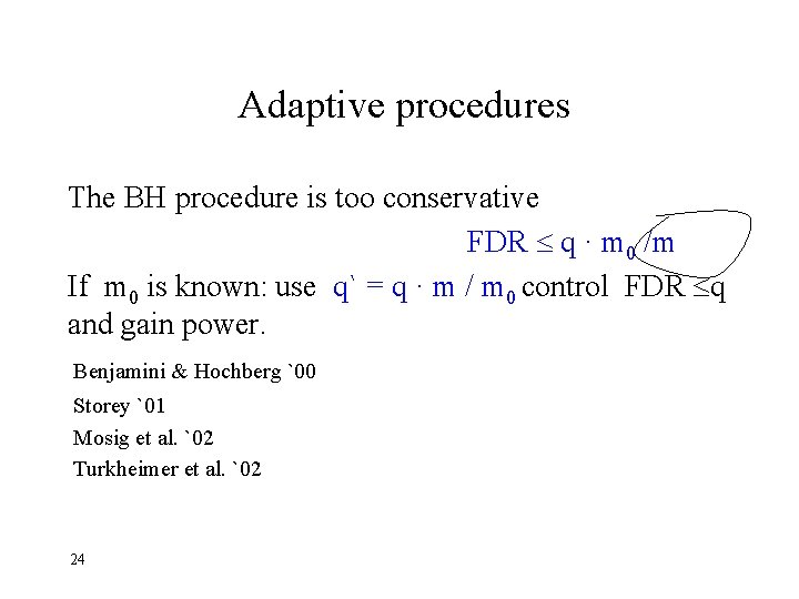
Adaptive procedures The BH procedure is too conservative FDR q · m 0 /m If m 0 is known: use q` = q · m / m 0 control FDR q and gain power. Benjamini & Hochberg `00 Storey `01 Mosig et al. `02 Turkheimer et al. `02 24

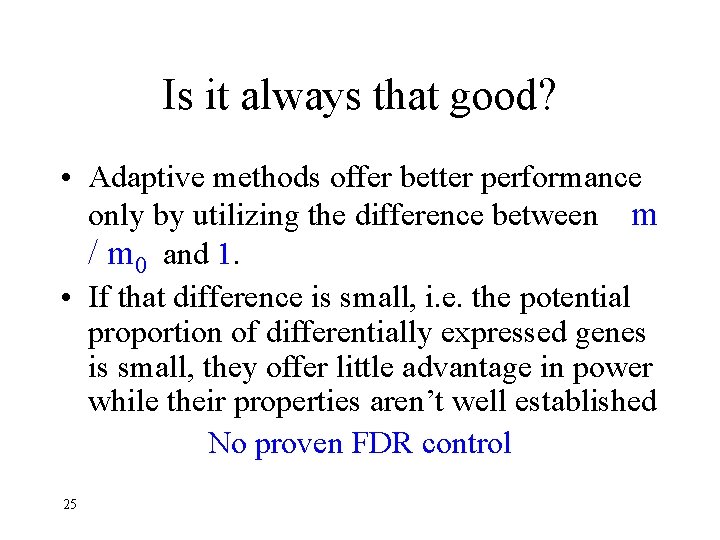
Is it always that good? • Adaptive methods offer better performance only by utilizing the difference between m / m 0 and 1. • If that difference is small, i. e. the potential proportion of differentially expressed genes is small, they offer little advantage in power while their properties aren’t well established No proven FDR control 25

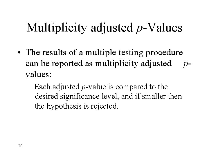
Multiplicity adjusted p-Values • The results of a multiple testing procedure can be reported as multiplicity adjusted pvalues: Each adjusted p-value is compared to the desired significance level, and if smaller then the hypothesis is rejected. 26

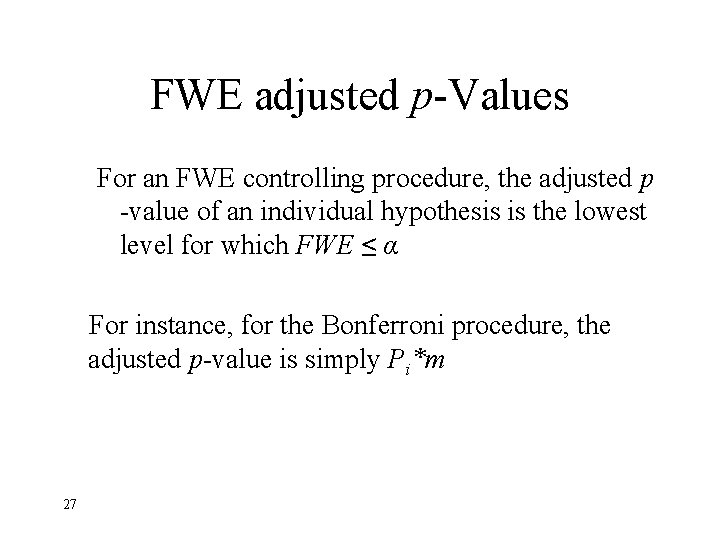
FWE adjusted p-Values For an FWE controlling procedure, the adjusted p -value of an individual hypothesis is the lowest level for which FWE ≤ α For instance, for the Bonferroni procedure, the adjusted p-value is simply Pi*m 27

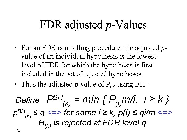
FDR adjusted p-Values • For an FDR controlling procedure, the adjusted pvalue of an individual hypothesis is the lowest level of FDR for which the hypothesis is first included in the set of rejected hypotheses. • Thus the adjusted p-value of P(k) using BH : Define PBH(k) = min { P(i)m/i, i ≥ k } p. BH(k) ≤ q <=> for some i ≥ k, p(i) ≤ qi/m <=> H(k) is rejected at FDR level q 28

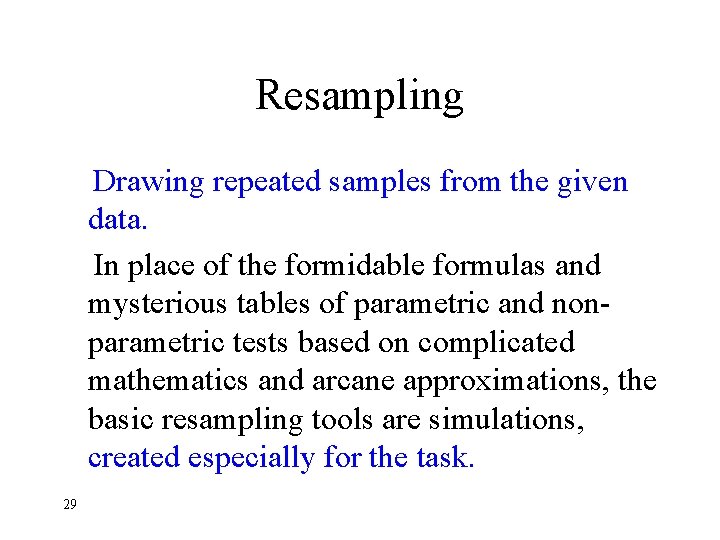
Resampling Drawing repeated samples from the given data. In place of the formidable formulas and mysterious tables of parametric and nonparametric tests based on complicated mathematics and arcane approximations, the basic resampling tools are simulations, created especially for the task. 29

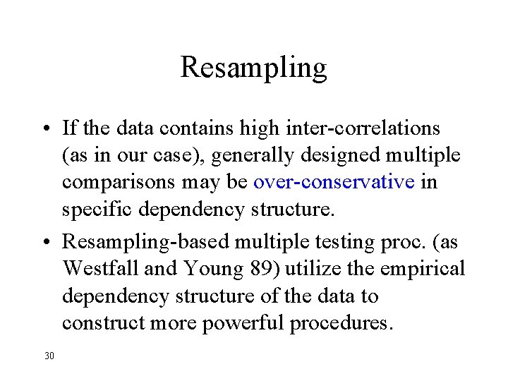
Resampling • If the data contains high inter-correlations (as in our case), generally designed multiple comparisons may be over-conservative in specific dependency structure. • Resampling-based multiple testing proc. (as Westfall and Young 89) utilize the empirical dependency structure of the data to construct more powerful procedures. 30

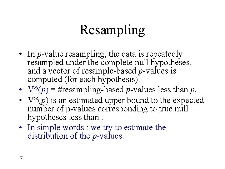
Resampling • In p-value resampling, the data is repeatedly resampled under the complete null hypotheses, and a vector of resample-based p-values is computed (for each hypothesis). • V*(p) = #resampling-based p-values less than p. • V*(p) is an estimated upper bound to the expected number of p-values corresponding to true null hypotheses less than. • In simple words : we try to estimate the distribution of the p-values. 31

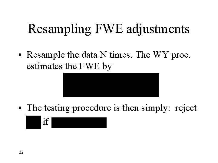
Resampling FWE adjustments • Resample the data N times. The WY proc. estimates the FWE by • The testing procedure is then simply: reject if 32

Resampling FDR adjustments • But FDR is also a function of the number of false null hypotheses being rejected. FDRest(p) = E { V*(p) / V*(p) + s(p) } s(p) = #false null hypotheses less than p Do we know s(p) ? No. But we can try and estimate it! 33

Estimation methods The two next methods use resampling to estimate the joint distribution of the p-values. ü The FDR local (point) estimator is conservative on the mean. ü The FDR upper limit bounds the FDR with probability 95%. More strict than the first method, and therefore less powerful. In the other hand it controls the empirical FDR with probability 0. 95, hence supplies more protection. 34

Alternative Estimation method ü Let’s use the BH procedure, but rather than using the raw p-values corresponding to the test statistics, the p-values are estimated by resampling from the marginal distribution and collapsing over all hypotheses. In simple words: averaging over all the genes, and then find the adjusted p-values and compare to q. The gain: It overcomes the discrete nature of the permutation distribution of a test statistics based on few observations (supply more possible values for the p-values). 35

If you insist then formally: For the k-th gene, with an observed test statistics tk , while N = #iterations and I = #genes, the estimated p-value is: And then obtain the BH point estimate for the k-th gene: 36

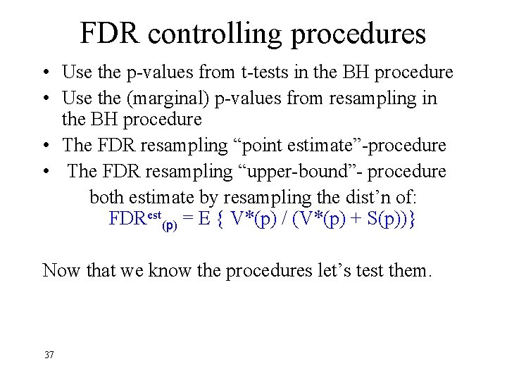
FDR controlling procedures • Use the p-values from t-tests in the BH procedure • Use the (marginal) p-values from resampling in the BH procedure • The FDR resampling “point estimate”-procedure • The FDR resampling “upper-bound”- procedure both estimate by resampling the dist’n of: FDRest(p) = E { V*(p) / (V*(p) + S(p))} Now that we know the procedures let’s test them. 37

The data Dudoit, Yang, Callow, Speed (2000): Statistical analysis of a lipid metabolism study in mice. • Treatment: 8 low HDL level knockout mice • Control: 8 “normal” C 57 B 1/6 mice • Purpose: Identification of single differentially expressed genes in the livers of mice with very low HDL cholesterol levels (treatment groups) compared to inbred control mice 38

• The micro-array data consists of 6359 genes. • Data was suitably standardized using log transformation and lowess smoother. • Compare gene expression means between the control and treatment groups. 39

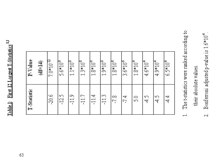
Results of multiple testing on the original data • The p-values obtained directly from the “raw” t-statistics with 14 degrees of freedom. Ignoring multiplicity, the actual number of raw p-values larger than 0. 05 is 568 (out of 6, 359). Let’s examine the FWE control in this case 40

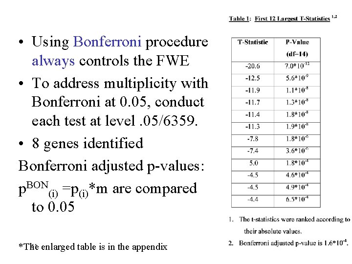
• Using Bonferroni procedure always controls the FWE • To address multiplicity with Bonferroni at 0. 05, conduct each test at level. 05/6359. • 8 genes identified Bonferroni adjusted p-values: p. BON(i) =p(i)*m are compared to 0. 05 41 enlarged table is in the appendix *The

• Applying the FDR controlling BH on the raw pvalues, we came up with the same 8 rejected null hypotheses obtained in the original analysis. Surprising ? Not really. Take a look at the table and observe the large gap between the p-values of genes identified by the FWE controlling procedure and the other p-values. Also don’t forget the actual distribution of the test statistics is not quite the same t-distribution underlying the derivation of the p-values. So what’s the next improvement? You know it. 42

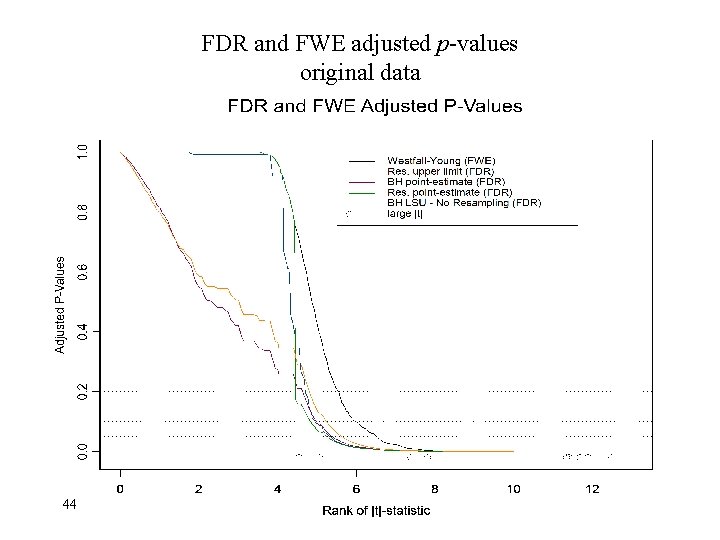
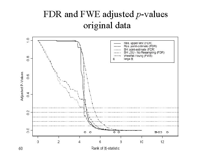
That’s right: Resampling • Let’s estimate the distribution of the t-statistics over 1000 resampling iterations. • Adjusted p-values were calculated using the WY alg. (FWE & resampling) and the 3 resampling-based procedures we learned. • The ten highest absolute t-values (except the largest one, 20. 6, which is too far outside of the plotted x-axis) are marked on the added plot. • At the 0. 05 significance level, we may still reject the same 8 hypotheses by all procedures. What about 0. 1? *The enlarged graph is in the appendix 43

FDR and FWE adjusted p-values original data 44

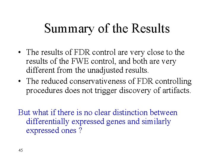
Summary of the Results • The results of FDR control are very close to the results of the FWE control, and both are very different from the unadjusted results. • The reduced conservativeness of FDR controlling procedures does not trigger discovery of artifacts. But what if there is no clear distinction between differentially expressed genes and similarly expressed ones ? 45

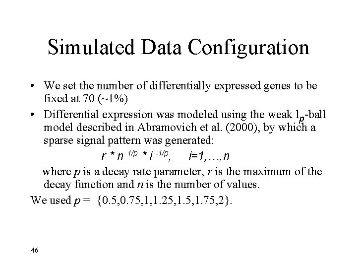
Simulated Data Configuration • We set the number of differentially expressed genes to be fixed at 70 (~1%) • Differential expression was modeled using the weak lp-ball model described in Abramovich et al. (2000), by which a sparse signal pattern was generated: r * n 1/p * i -1/p, i=1, …, n where p is a decay rate parameter, r is the maximum of the decay function and n is the number of values. We used p = {0. 5, 0. 75, 1, 1. 25, 1. 75, 2}. 46

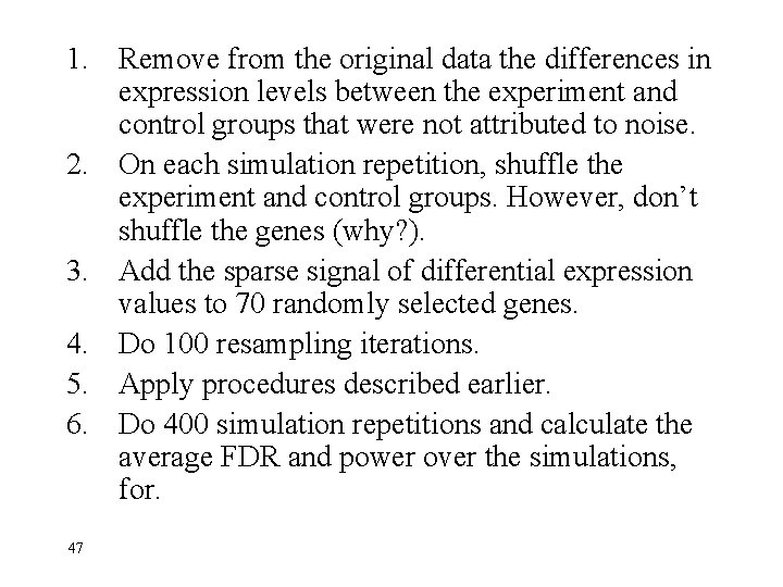
1. Remove from the original data the differences in expression levels between the experiment and control groups that were not attributed to noise. 2. On each simulation repetition, shuffle the experiment and control groups. However, don’t shuffle the genes (why? ). 3. Add the sparse signal of differential expression values to 70 randomly selected genes. 4. Do 100 resampling iterations. 5. Apply procedures described earlier. 6. Do 400 simulation repetitions and calculate the average FDR and power over the simulations, for. 47

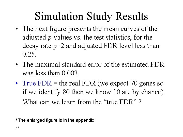
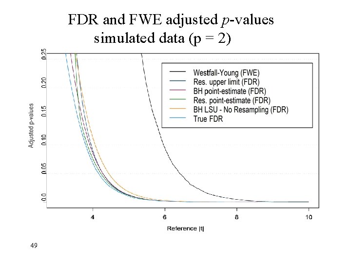
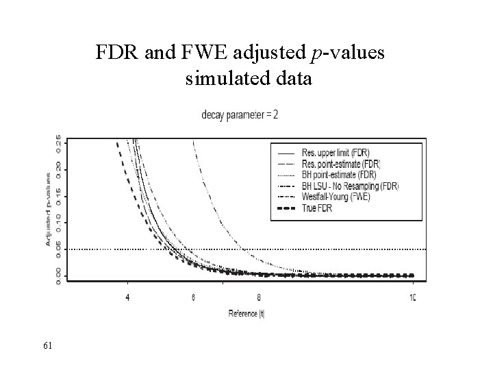
Simulation Study Results • The next figure presents the mean curves of the adjusted p-values vs. the test statistics, for the decay rate p=2 and adjusted FDR level less than 0. 25. • The maximal standard error of the estimated FDR was less than 0. 003. • True FDR = the real FDR (we expect 70 genes so if we identify 80 then we know 10 are by chance). What can we learn from the “true FDR” ? *The enlarged figure is in the appendix 48

FDR and FWE adjusted p-values simulated data (p = 2) 49

What can we learn from the “true FDR” ? • For all FDR controlling procedures, the adjusted p -values are larger then the corresponding true FDR, indicating that using them guarantees the control of the FDR. • The FDR procedures produce FDR adjusted pvalues much closer to the true FDR than the FWE adjusted p-values obtained by the WY alg. 50

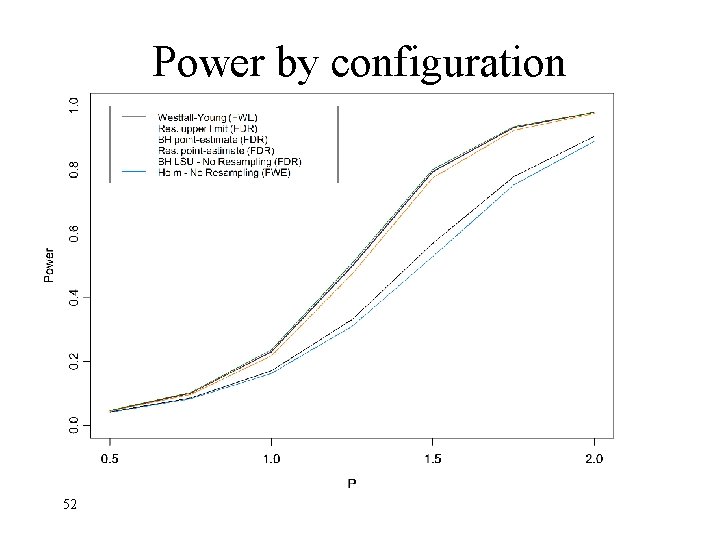
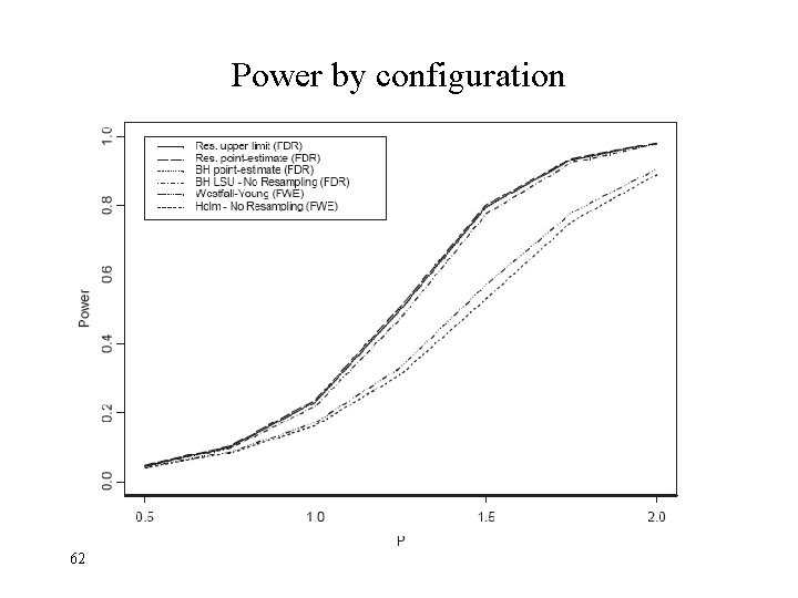
What about the power? • Here we also include Holm’s non-resampling multiple testing procedure, which controls the FWE. • All FDR controlling procedures obtain substantially more power than the FWE controlling procedures. • Pay attention for the differences of resampling and non-resampling proc. *The enlarged figure is in the appendix 51

Power by configuration 52

Power • The resampling point-estimator is the most powerful procedure • The other two resampling estimators following very closely behind. Although the upper-limit res. estimates the joint distribution of the test statistics, its relative conservativeness does not allow increase of power over the BH resampling est. , which estimates only the marginal distribution. 53

Power • The BH linear step-up procedure performs relatively well, in spite of it assuming tdistributed test statistics that are either independent or positively dependent, and not using resampling. • Holm’s procedure, performing the most poorly, reconfirms the advantage of resampling for cases in which the test statistics are not independent. 54

Discussion • Why limiting the power to generate candidate hypotheses at this stage? • Controlling the FDR at the screening stage of the research carries a benefit for the next stages of the analysis (and then we can use FWE or FDR for the follow-up studies) 55

• It is not quite clear how the dependency structure affects the performance of multiple testing procedures. Measurement error of microarray data tends to be positively dependent. • A co-regulation dependency may be a result of biological variability of the co-regulation and need not be positive. • Characterization of the dependency structure attributed to the above common co-regulation is one of the main research targets of micro-array experiments. • Pre-selections of genes that pass an initial FDR testing at not too low level can suppress noise? 56

Summary • We learned four procedures that were shown to control the FDR at the desired level • Clearly, all FDR controlling procedures retain higher power than FWE controlling procedures, and are therefore highly useful for the discovery of differential genetic expression. • The choice among the four is a matter of buying more power and better properties at the expense of more complicated computations. • Substantial increase in power is already gained when the p-values are estimated by resampling 57

Thanks Yoav Benjamini Anat Reiner Note: On the course site you can watch this presentation along with the added notes to the slides which will help you to understand it even better. 58

Appendix 59

FDR and FWE adjusted p-values original data 60

FDR and FWE adjusted p-values simulated data 61

Power by configuration 62

63