EFFICIENT NUMERICAL METHODS FOR PHASEFIELD EQUATIONS Tao Tang

EFFICIENT NUMERICAL METHODS FOR PHASE-FIELD EQUATIONS Tao Tang Hong Kong Baptist University September 11 -13， 2013 Russian-Chinese Workshop on Numer Analysis and Scientific Computing

John W. Cahn (1928 -- ) John E. Hilliard (1826 -1987) The Cahn-Hilliard equation: describes the process of phase separation:

Microstructural evolution under the Cahn–Hilliard equation, demonstrating distinctive coarsening and phase separation.

PHYSICS Cahn-Hilliard equation Phase separation in a binary alloy (metal, liquid, …) Spinodal decomposition Mass conservation Interface minimization

MATHEMATICS

HIGH-ORDER NONLINEAR DIFFUSION EQUATIONS: How to do time integration? If both dynamics and steady state are required，how to do efficient time discretization? Higher order methods vs. efficiency; Adaptivity

EXAMPLES OF HIGH ORDER NONLINEAR DIFFUSION EQUATION Molecular Beam Epitaxy (MBE) Model [T. , Xu; WB Chen et ] Inpaiting with Cahn-Hilliard Equation [A. L. Bertozzi, etc] Phase field crystal equation [Lowengrub, Wang, Wise etc] Thin Film epitaxy [J. Shen, X. M. Wang, Wise, etc]

EXAMPLE Cahn-Hilliard impainting [Bertozzi etc. IEEE Tran. Imag. Proc. 2007, Commun. Math. Sci, 2011] Monotonic decrease of the energy functional during the coarsening process

NUMERICAL CHALLENGES Interior layers (i. e. thin interface) see a figure Time discretization: Lower order (good for stability)? “h”-adaptivity; “p”-adaptivity?

Thin-film epitaxy without slope selection Energy Cahn-Hilliard equation Energy Allen-Cahn equation Energy curves of three different models

EXAMPLE Consider the IBV problem for the Cahn-Hilliard Eq. Explicit Euler’s scheme (10 -7) Semi-implicit Euler’s scheme (10 -4) Implicit Euler’s scheme (10 -6)! Non-linearly stabilized scheme (implicit for the biharmonic and non-linear terms : -- 10 -3) Linearly stabilized splitting scheme: introducing two splitting functionals; one is contractive and the other is expansive: (10 -2 ~ 10 -3)

A STABLE FIRST-ORDER METHOD:

Eyre’s method Convexity splitting where and are strictly convex. The semiimplicit discretization is given by Various Eyre’s type or various extension: Inpaiting problem [Schönlieb & Bertozzi] Coarsening simulations [Vollmayr-Lee & Rutenberg] Second-order convex splitting [J. Shen, C. Wang, Wise] Question: Given Eyre’s GS scheme, can we use some iterative ideas to obtain a higher order semi-stable method?

SPECTRAL DEFERRED CORRECTION (SDC) FOR Y’=F(T, Y) The method is introduced by Dutt, Greengard and Rokhlin (BIT, 2000) Multi-implicit SDC method (Layton and Minion, 2004) SDC with high-order RK schemes [Christliek, Qiu and Ong, 2010] Collocation Method:

Algorithm (SDC method) 1 (Prediction). Use a k 0 -th order numerical method to compute 2 (Correction). For j=1, …, J l Compute the residual for l Define the error function for l Form the error equation l Use an k-th order method to compute at the grid points tn, i on [tn, tn+1]. l Define a new approximation solution

CONVERGENCE ANALYSIS [T. , H. -H. XIE, X. -B. YIN, JSC 2012] Theorem 1: Let be computed in the Correction step of the SDC Algorithm. If the step-size h is sufficiently small, then the following error estimate holds:

Outline Note

Algorithm (Modified SDC method) : Same as Algorithm 1, except that after is computed we use some Picard smoothing After the above k-1 iterations, let Theorem 2 Let be computed in the Correction step of the modified SDC Algorithm. If the step size h is sufficiently small, and if special collocation points (e. g. Gauss) are used, then

Proof. It follows from (S 1) that

Efficiency comparison using Legendre-Gauss quadrature nodes

Energy evolutions with different time steps

FIRST-ORDER LINEAR SCHEME Simple, linear discretization in time; First-order with energy decreasing; In space, central differencing FFT is used

STABILTY+ACCURACY VIA P-ADAPTIVITY Use Energy difference at and steps If the difference is small, no correction; If the difference is large, judge how many SDC corrections are needed. Note most of time regimes, no corrections are needed

fine sh e m coarse mesh with correction

Energy evolutions with different time steps and different numbers of corrections for the Cahn-Hilliard equation

Blowing up phenomenon of semi-implicit spectral deferred correction with uniform number of corrections

HOW MANY ITERATIONS NEEDED

Energy curves of the thin film model without slope selection and number of corrections CPU time comparison

ADAPTIVE TIME STEPPING: Energy is an important physical quantity to reflect the structure evolution. Adaptive time step is determined by ∆tmin corresponds to quick evolution of the solution, while ∆tmax to slow evolution. [Qiao, T. , Zhang, SISC, 2010]

TIME ADAPTIVITY VIA ENERGY VARIATION (XIE; T. , LUO) Numerical Scheme for C-H eqn: Stability: Discrete energy identity:

Equi-energy: • It follows from the numerical scheme and the energy identity that • The prescribed energy decrease ( ) equation • Time stepping formula • One step fix-point iteration to solve the prescribed energy decrease equation

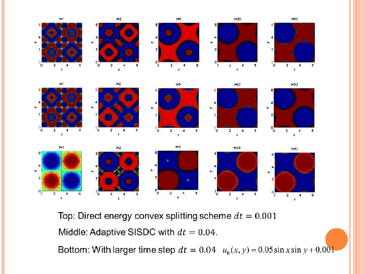
The initial condition is random in [-0. 1, 0. 1], with periodic boundary condition and

EXAMPLE [ARTIFICIAL DISSIPPATION] MOLECULAR BEAN EPITAXY (MBE) MODEL: Model eqn: ht = - 2 h - [ (1 - | h|2) h ] Energy identity: where

ARTIFICIAL DISSIPATION: Remedy: i. e. an O( t) is added, where A > 0 is an O(1) constant. Property: If the constant A is sufficiently large, then E(hn+1) E(hn)? If the numerical solution is convergent, then the condition for A is T & C. Xu: [SINUM, 2006]

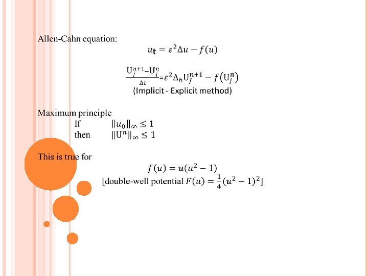
MORE ON REGULARITY: Consider the nonlinear 2 -D model for epitaxial growth of thin films: Here, we prove an a-priori bound on the L -norm of h in the 2 -D case with =0. The proof heavily relies on the maximum principle. It is hard to see how it can be extended to the case of (small) positive . However, it is intuitively clear that in the case of positive , the solution should be more regular, and one may expect that the similar bound on h still holds.

CONCLUSIONS/REMARKS High-order time discretization is needed for high-order nonlinear diffusion equations. The use of the SDC method seems a useful way. Analysis of nonlinear stability and convergence require deep understanding of the relevant PDEs and numerical methods. [local estimates … T. & Xu SINUM 2006, Bertozzi etc] The analysis for adaptive schemes is highly nontrivial. Most of the existing numerical methods are lack of rigorous mathematical justification.

THANKS! HTTP: //WWW. MATH. HKBU. EDU. HK/~TTANG