Efficient experimentation for nanostructure synthesis using Sequential Minimum

Efficient experimentation for nanostructure synthesis using Sequential Minimum Energy Designs (SMED) V. Roshan Joseph+, Tirthankar Dasgupta* and C. F. Jeff Wu+ + ISy. E, Georgia Tech *Statistics, Harvard 1

Statistical modeling and analysis for robust synthesis of nanostructures l Dasgupta, Ma, Joseph, Wang and Wu (2008), Journal of The American Statistical Association, to appear. l Robust conditions for synthesis of Cadmium Selenide (Cd. Se) nanostructures derived l l New sequential algorithm for fitting multinomial logit models. Internal noise factors considered. 2

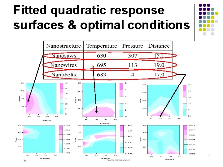
Fitted quadratic response surfaces & optimal conditions 3

The need for more efficient experimentation l A 9 x 5 full factorial experiment was too expensive and time consuming. l Quadratic response surface did not capture nanowire growth satisfactorily (Generalized R 2 was 50% for Cd. Se nanowire sub-model). 4

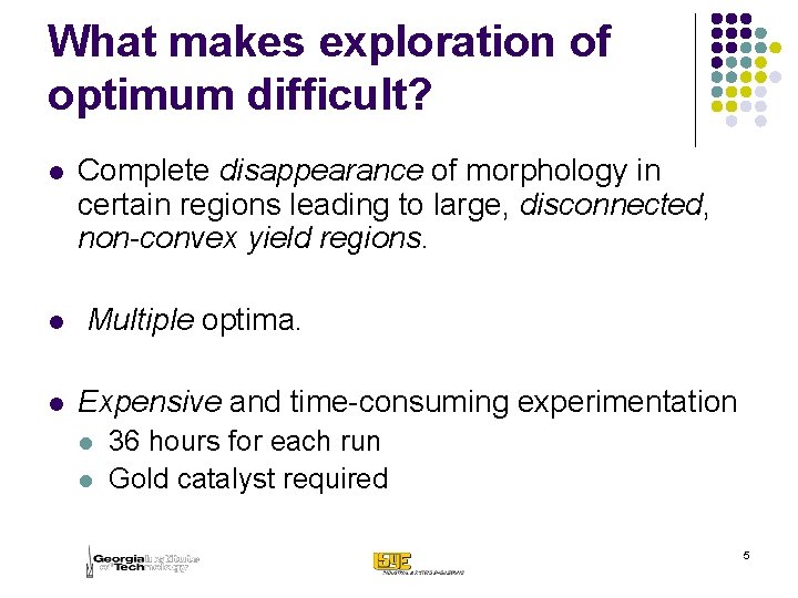
What makes exploration of optimum difficult? l l l Complete disappearance of morphology in certain regions leading to large, disconnected, non-convex yield regions. Multiple optima. Expensive and time-consuming experimentation l l 36 hours for each run Gold catalyst required 5

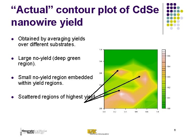
“Actual” contour plot of Cd. Se nanowire yield l Obtained by averaging yields over different substrates. l Large no-yield (deep green region). l Small no-yield region embedded within yield regions. l Scattered regions of highest yield. 6

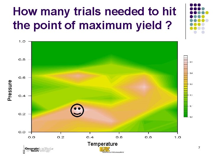
Pressure How many trials needed to hit the point of maximum yield ? Temperature 7

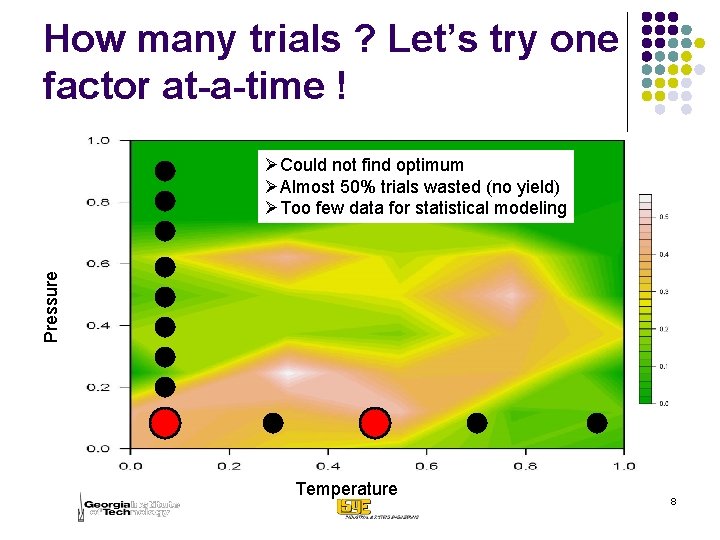
How many trials ? Let’s try one factor at-a-time ! Pressure ØCould not find optimum ØAlmost 50% trials wasted (no yield) ØToo few data for statistical modeling Temperature 8

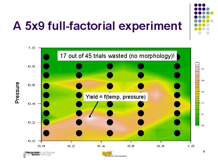
A 5 x 9 full-factorial experiment Pressure 17 out of 45 trials wasted (no morphology)! Yield = f(temp, pressure) 9

Why are traditional methods inappropriate ? l l Need a sequential approach to keep run size to a minimum. Fractional factorials / orthogonal arrays l l Large number of runs as number of levels increase. Several no-morphology scenarios possible. Do not facilitate sequential experimentation. Response Surface Methods l l Complexity of response surface. Categorical (binary in the extreme case) possible. 10

The Objective l To find a design strategy that l l Is model-independent, Can “carve out’’ regions of no-morphology quickly, Allows for exploration of complex response surfaces, Facilitates sequential experimentation. 11

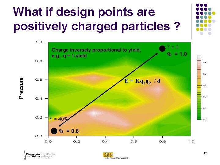
What if design points are positively charged particles ? Pressure Charge inversely proportional to yield, e. g. , q = 1 -yield Y=0 q 2 = 1. 0 E = Kq 1 q 2 / d Y = 40% q 1 = 0. 6 12

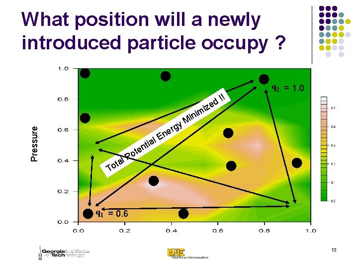
Pressure What position will a newly introduced particle occupy ? al i t n tal o T E rgy e n !! d ize m ni i M q 2 = 1. 0 te o P q 1 = 0. 6 13

The key idea l l l Pick a point x. Conduct experiment at x and observe yield y(x). Assign charge q(x) inversely proportional to y(x) l l How quickly will you reach the optimum ? Once you reach there, how will you know that THIS IS IT ? Use y(x) to update your knowledge about yields at various points in the design space (How ? ) Pick the next point as the one that minimizes the total potential energy in the design space. 14

The SMED algorithm 15

The next design point 16

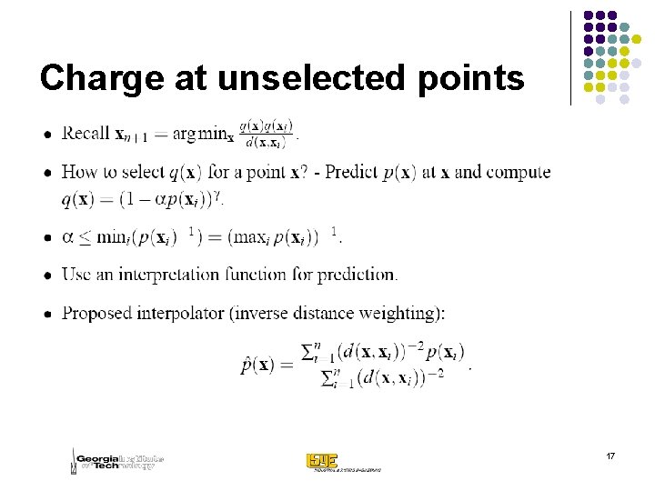
Charge at unselected points 17

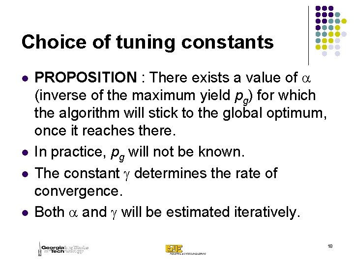
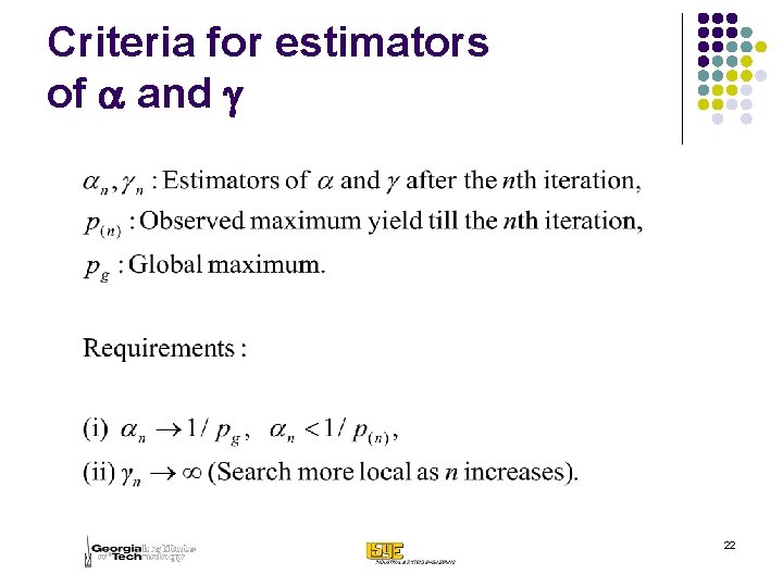
Choice of tuning constants l l PROPOSITION : There exists a value of a (inverse of the maximum yield pg) for which the algorithm will stick to the global optimum, once it reaches there. In practice, pg will not be known. The constant g determines the rate of convergence. Both a and g will be estimated iteratively. 18

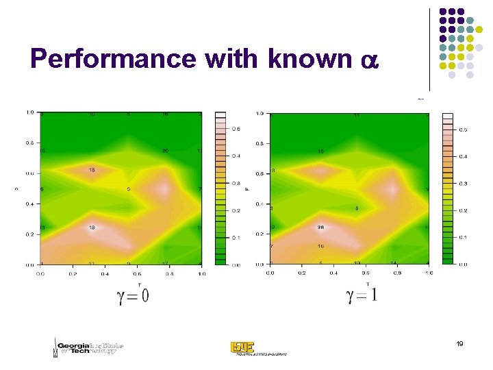
Performance with known a 19

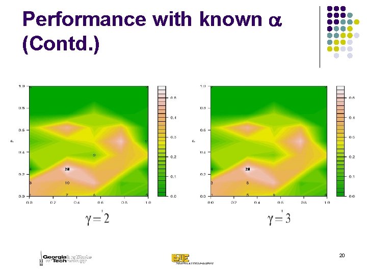
Performance with known a (Contd. ) 20

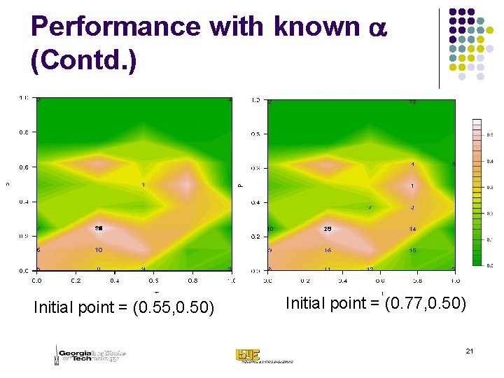
Performance with known a (Contd. ) Initial point = (0. 55, 0. 50) Initial point = (0. 77, 0. 50) 21

Criteria for estimators of a and g 22

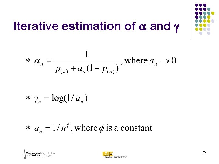
Iterative estimation of a and g 23

Improved SMED for random response l l Instead of an interpolating function, use a smoothing function to predict yields (and charges) at unobserved points. Update the charges of selected points as well, using the smoothing function. Local polynomial smoothing used. Two parameters: l l n. T (threshold number of iterations after which smoothing is started). l (smoothing constant; small l: local fitting). 24

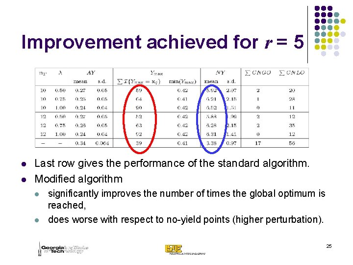
Improvement achieved for r = 5 l l Last row gives the performance of the standard algorithm. Modified algorithm l l significantly improves the number of times the global optimum is reached, does worse with respect to no-yield points (higher perturbation). 25

Summary l l l A new sequential space-filling design SMED proposed. SMED is model independent, can quickly “carve out” no-morphology regions and allows for exploration of complex surfaces. Origination from laws of electrostatics. Algorithm for deterministic functions. Modified algorithm for random functions. Performance studied using nanowire data, modified Branin (2 dimensional) and Levy-Montalvo (4 dimensional) functions. 26

Predicting the future Use my SMED ! What the hell! I don’t want to use this stupid strategy for experimentation ! Stat Nano Image courtesy : www. cartoonstock. com 27

28

Advantages of space filling designs l l l LHD (Mc. Cay et al. 1979), Uniform designs (Fang 2002) are primarily used for computer experiments. Can be used to explore complex surfaces with small number of runs. Model free. No problems with categorical/binary data. CAN THEY l BE USED FOR SEQUENTIAL EXPERIMENTATION ? l CARVE OUT REGIONS OF NO-MORPHOLOGY QUICKLY? 29

Sequential experimentation strategies for global optimization l l SDO, a grid-search algorithm by Cox and John (1997) l Initial space-filling design. l Prediction using Gaussian Process Modeling. l Lower bounds on predicted values used for sequential selection of evaluation points. Jones, Schonlau and Welch (1998) l Similar to SDO. l Expected Improvement (EI) Criterion used. l Balances the need to exploit the approximating surface with the need to improve the approximation. 30

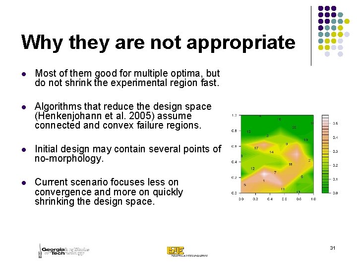
Why they are not appropriate l Most of them good for multiple optima, but do not shrink the experimental region fast. l Algorithms that reduce the design space (Henkenjohann et al. 2005) assume connected and convex failure regions. l Initial design may contain several points of no-morphology. l Current scenario focuses less on convergence and more on quickly shrinking the design space. 31

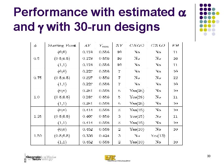
Some performance measures for n 0 - run designs. 32

Performance with estimated a and g with 30 -run designs 33

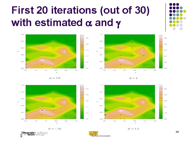
First 20 iterations (out of 30) with estimated a and g 34

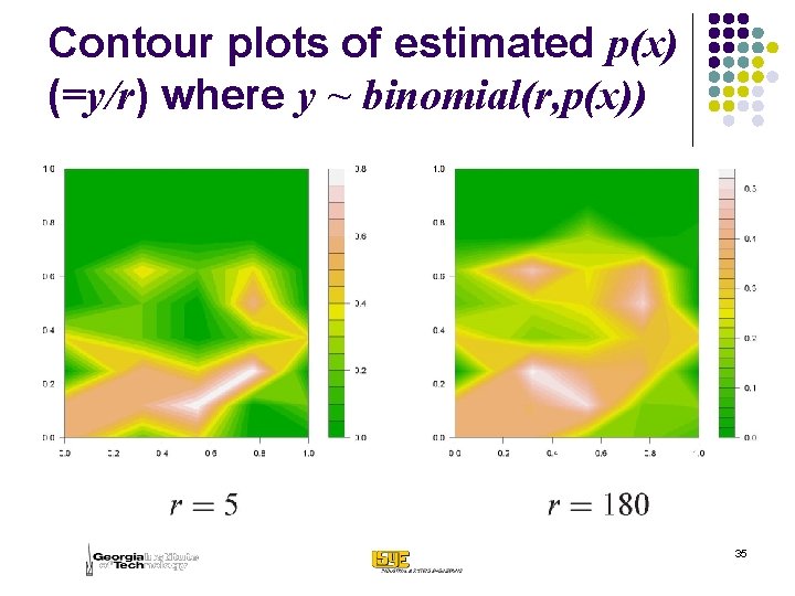
Contour plots of estimated p(x) (=y/r) where y ~ binomial(r, p(x)) 35

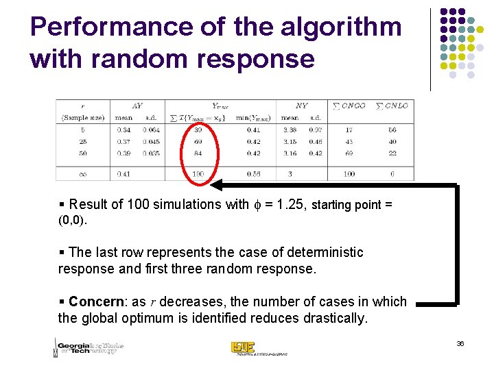
Performance of the algorithm with random response § Result of 100 simulations with f = 1. 25, starting point = (0, 0). § The last row represents the case of deterministic response and first three random response. § Concern: as r decreases, the number of cases in which the global optimum is identified reduces drastically. 36