ECE 352 Systems II Manish K Gupta Ph

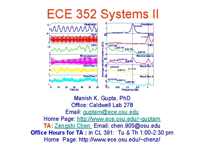
ECE 352 Systems II Manish K. Gupta, Ph. D Office: Caldwell Lab 278 Email: guptam@ece. osu. edu Home Page: http: //www. ece. osu. edu/~guptam TA: Zengshi Chen Email: chen. 905@osu. edu Office Hours for TA : in CL 391: Tu & Th 1: 00 -2: 30 pm Home Page: http: //www. ece. osu. edu/~chenz/

Acknowledgements • Various graphics used here has been taken from public resources instead of redrawing it. Thanks to those who have created it. • Thanks to Brian L. Evans and Mr. Dogu Arifler • Thanks to Randy Moses and Bradley Clymer

Fourier Transform ECE 352

ECE 352 REVIEW SOME CONCEPTS Slides edited from: • Prof. Brian L. Evans and Mr. Dogu Arifler Dept. of Electrical and Computer Engineering The University of Texas at Austin course: EE 313 Linear Systems and Signals Fall 2003

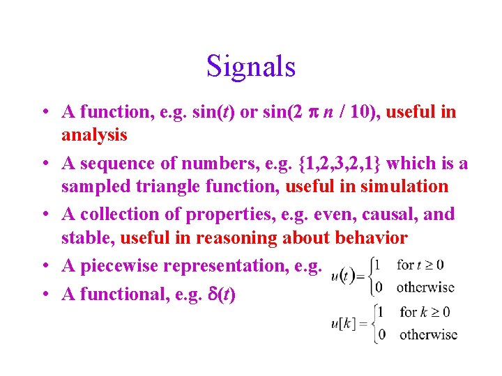
Signals • A function, e. g. sin(t) or sin(2 p n / 10), useful in analysis • A sequence of numbers, e. g. {1, 2, 3, 2, 1} which is a sampled triangle function, useful in simulation • A collection of properties, e. g. even, causal, and stable, useful in reasoning about behavior • A piecewise representation, e. g. • A functional, e. g. d(t)

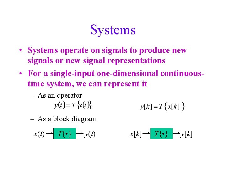
Systems • Systems operate on signals to produce new signals or new signal representations • For a single-input one-dimensional continuoustime system, we can represent it – As an operator – As a block diagram x(t) T{ • } y(t) x[k] T{ • } y[k]

System Properties • Let x[k], x 1[k], and x 2[k] be inputs to a linear system and let y[k], y 1[k], and y 2[k] be their corresponding outputs • A linear system satisfies – Additivity: x 1[k] + x 2[k] y 1[k] + y 2[k] – Homogeneity: a x[k] a y[k] for any constant a • Let x[k] be the input to time-invariant system and y[k] be its corresponding output. Then, x[k - m] y[k - m], for any integer m

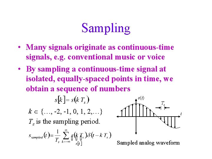
Sampling • Many signals originate as continuous-time signals, e. g. conventional music or voice • By sampling a continuous-time signal at isolated, equally-spaced points in time, we obtain a sequence of numbers s(t) Ts k {…, -2, -1, 0, 1, 2, …} Ts is the sampling period. t Sampled analog waveform

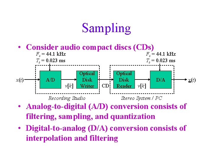
Sampling • Consider audio compact discs (CDs) Fs = 44. 1 k. Hz Ts = 0. 023 ms x(t) A/D v[k] Fs = 44. 1 k. Hz Ts = 0. 023 ms Optical Disk Writer Recording Studio CD Optical Disk Reader D/A v[k] Stereo System / PC • Analog-to-digital (A/D) conversion consists of filtering, sampling, and quantization • Digital-to-analog (D/A) conversion consists of interpolation and filtering x(t)

Laplace Transform

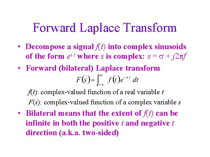
Forward Laplace Transform • Decompose a signal f(t) into complex sinusoids of the form es t where s is complex: s = s + j 2 pf • Forward (bilateral) Laplace transform f(t): complex-valued function of a real variable t F(s): complex-valued function of a complex variable s • Bilateral means that the extent of f(t) can be infinite in both the positive t and negative t direction (a. k. a. two-sided)

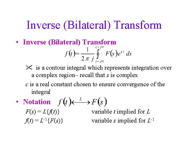
Inverse (Bilateral) Transform • Inverse (Bilateral) Transform is a contour integral which represents integration over a complex region– recall that s is complex c is a real constant chosen to ensure convergence of the integral • Notation F(s) = L{f(t)} f(t) = L-1{F(s)} variable t implied for L variable s implied for L-1

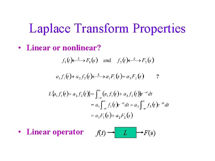
Laplace Transform Properties • Linear or nonlinear? • Linear operator f(t) L F(s)

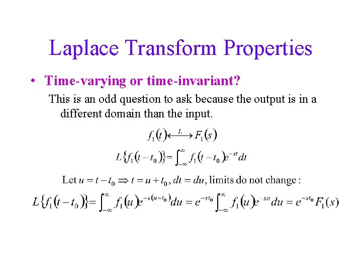
Laplace Transform Properties • Time-varying or time-invariant? This is an odd question to ask because the output is in a different domain than the input.

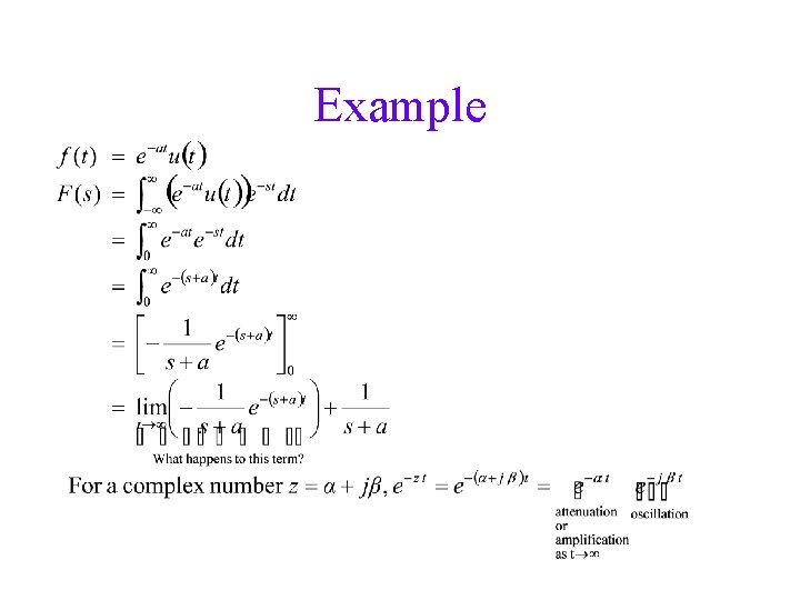
Example

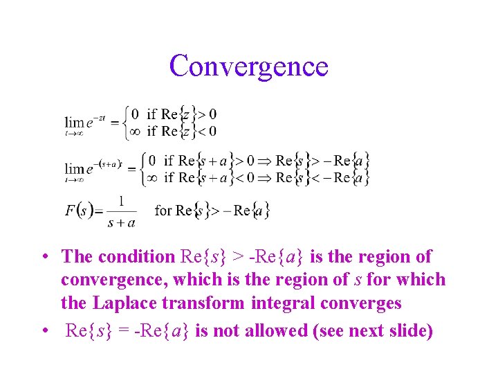
Convergence • The condition Re{s} > -Re{a} is the region of convergence, which is the region of s for which the Laplace transform integral converges • Re{s} = -Re{a} is not allowed (see next slide)

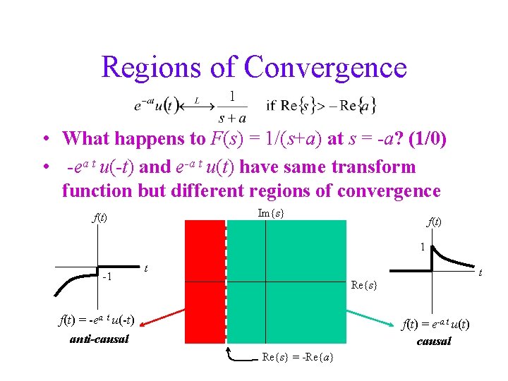
Regions of Convergence • What happens to F(s) = 1/(s+a) at s = -a? (1/0) • -ea t u(-t) and e-a t u(t) have same transform function but different regions of convergence Im{s} f(t) 1 -1 t t Re{s} f(t) = -ea t u(-t) f(t) = e-a t u(t) causal anti-causal Re{s} = -Re{a}

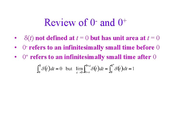
Review of 0 and + 0 • d(t) not defined at t = 0 but has unit area at t = 0 • 0 - refers to an infinitesimally small time before 0 • 0+ refers to an infinitesimally small time after 0

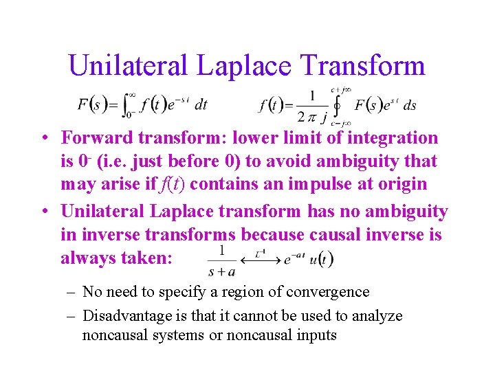
Unilateral Laplace Transform • Forward transform: lower limit of integration is 0 - (i. e. just before 0) to avoid ambiguity that may arise if f(t) contains an impulse at origin • Unilateral Laplace transform has no ambiguity in inverse transforms because causal inverse is always taken: – No need to specify a region of convergence – Disadvantage is that it cannot be used to analyze noncausal systems or noncausal inputs

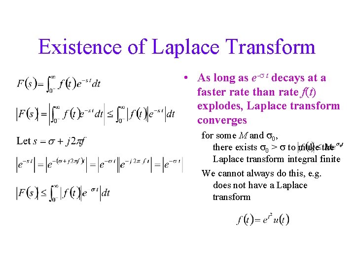
Existence of Laplace Transform • As long as e-s t decays at a faster rate than rate f(t) explodes, Laplace transform converges for some M and s 0, there exists s 0 > s to make the Laplace transform integral finite We cannot always do this, e. g. does not have a Laplace transform

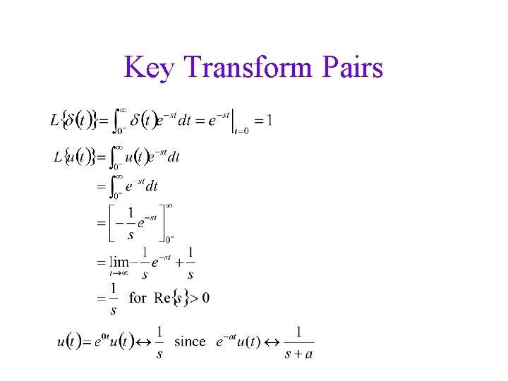
Key Transform Pairs

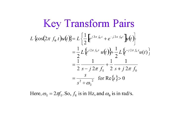
Key Transform Pairs

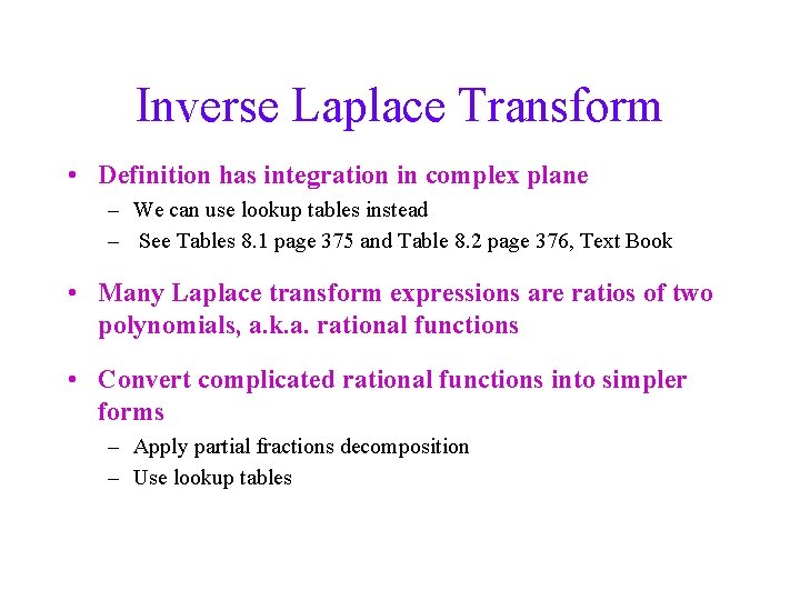
Inverse Laplace Transform • Definition has integration in complex plane – We can use lookup tables instead – See Tables 8. 1 page 375 and Table 8. 2 page 376, Text Book • Many Laplace transform expressions are ratios of two polynomials, a. k. a. rational functions • Convert complicated rational functions into simpler forms – Apply partial fractions decomposition – Use lookup tables

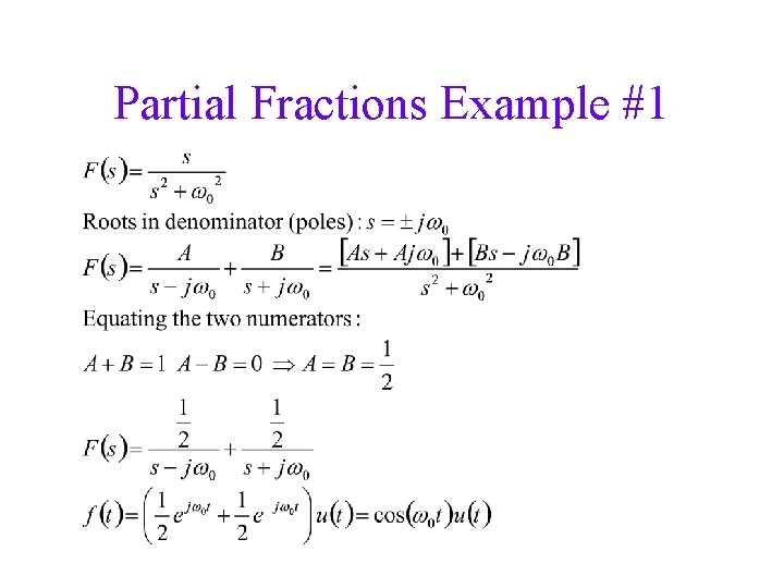
Partial Fractions Example #1

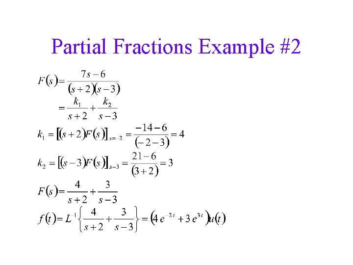
Partial Fractions Example #2

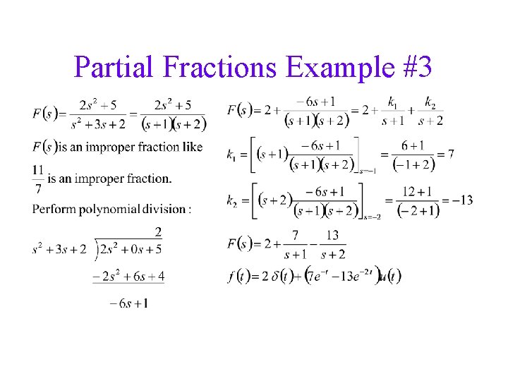
Partial Fractions Example #3

Use Matlab to find Laplace Transform, Inverse Laplace Transform ?

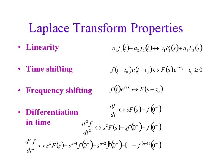
Laplace Transform Properties • Linearity • Time shifting • Frequency shifting • Differentiation in time

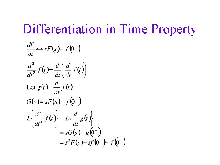
Differentiation in Time Property

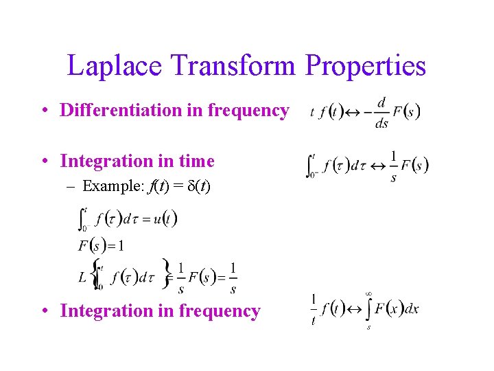
Laplace Transform Properties • Differentiation in frequency • Integration in time – Example: f(t) = d(t) • Integration in frequency

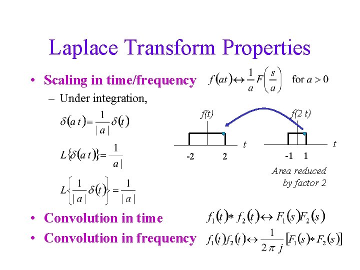
Laplace Transform Properties • Scaling in time/frequency – Under integration, f(2 t) f(t) t t -2 • Convolution in time • Convolution in frequency 2 -1 1 Area reduced by factor 2

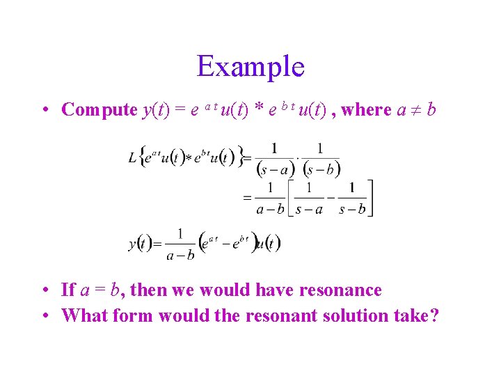
Example • Compute y(t) = e a t u(t) * e b t u(t) , where a b • If a = b, then we would have resonance • What form would the resonant solution take?

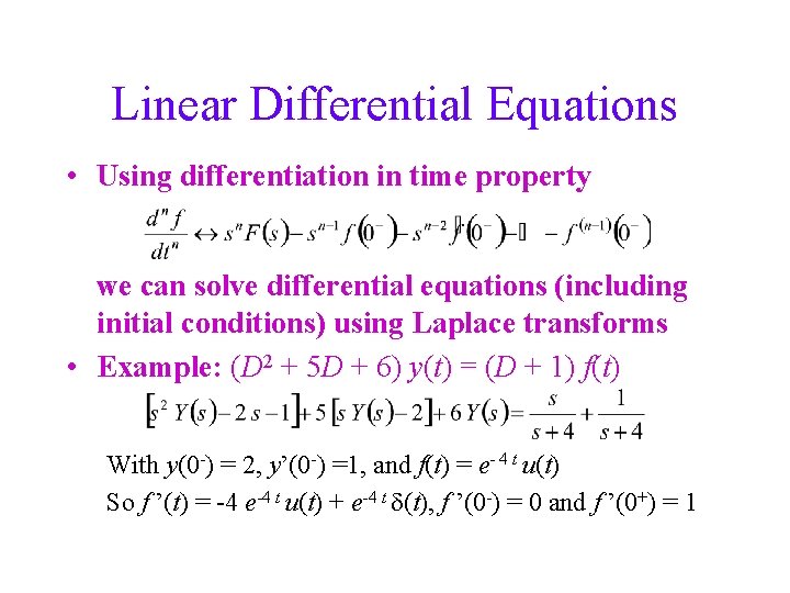
Linear Differential Equations • Using differentiation in time property we can solve differential equations (including initial conditions) using Laplace transforms • Example: (D 2 + 5 D + 6) y(t) = (D + 1) f(t) With y(0 -) = 2, y’(0 -) =1, and f(t) = e- 4 t u(t) So f ’(t) = -4 e-4 t u(t) + e-4 t d(t), f ’(0 -) = 0 and f ’(0+) = 1

3 rd Day Class Home Work No Submission • • Read Pages 363 -375 (Chapter 8) Play with Matlab !

Any Questions ?