Digital Speech Processing Homework 1 Discrete Hidden Markov

Digital Speech Processing Homework #1 Discrete Hidden Markov Model Implementation Date: Oct. 27, 2010 Revised by Tsung-Wei Tu

Outline HMM in Speech Recognition Problems of HMM ◦ Training ◦ Testing File Format Submit Requirement 2

HMM in Speech Recognition 3

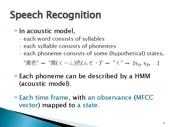
Speech Recognition In acoustic model, ◦ each word consists of syllables ◦ each syllable consists of phonemes ◦ each phoneme consists of some (hypothetical) states. “青色” → “青(ㄑㄧㄥ)色(ㄙㄜ、)” → ”ㄑ” → {s 1, s 2, …} Each phoneme can be described by a HMM (acoustic model). Each time frame, with an observance (MFCC vector) mapped to a state. 4

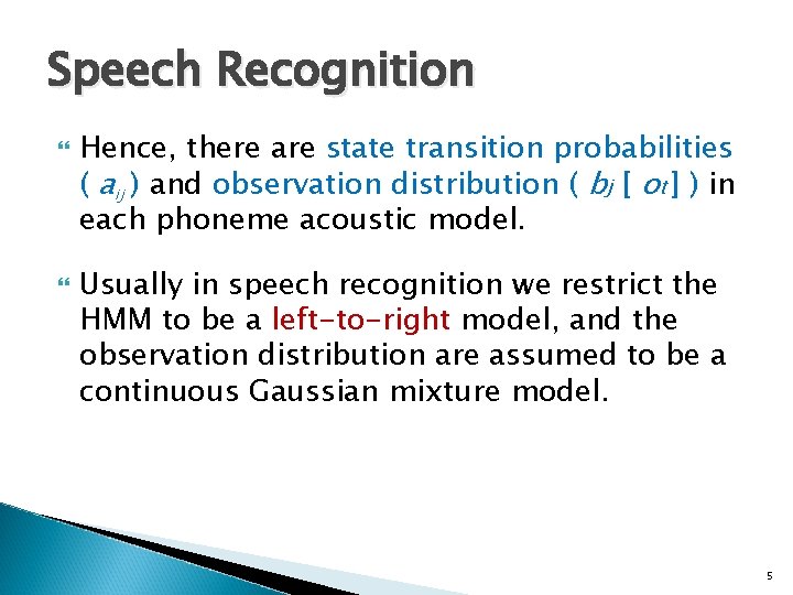
Speech Recognition Hence, there are state transition probabilities ( aij ) and observation distribution ( bj [ ot ] ) in each phoneme acoustic model. Usually in speech recognition we restrict the HMM to be a left-to-right model, and the observation distribution are assumed to be a continuous Gaussian mixture model. 5

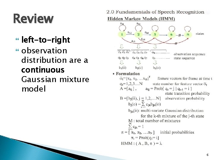
Review left-to-right observation distribution are a continuous Gaussian mixture model 6

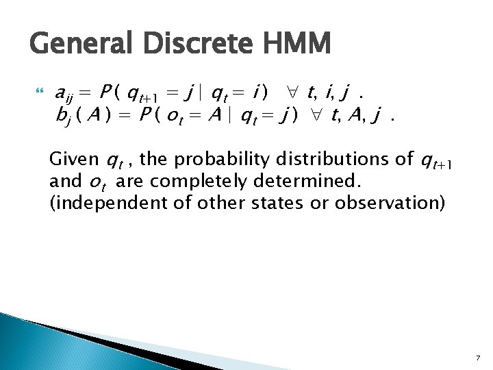
General Discrete HMM aij = P ( qt+1 = j | qt = i ) t, i, j. b j ( A ) = P ( o t = A | q t = j ) t, A , j. Given qt , the probability distributions of qt+1 and ot are completely determined. (independent of other states or observation) 7

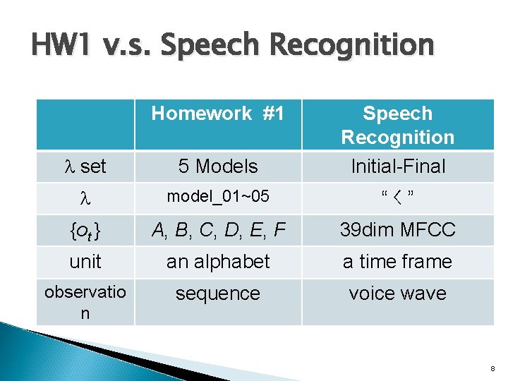
HW 1 v. s. Speech Recognition Homework #1 set 5 Models Speech Recognition Initial-Final model_01~05 “ㄑ” {ot } A, B, C, D, E, F 39 dim MFCC unit an alphabet a time frame observatio n sequence voice wave 8

Problems of HMM 9

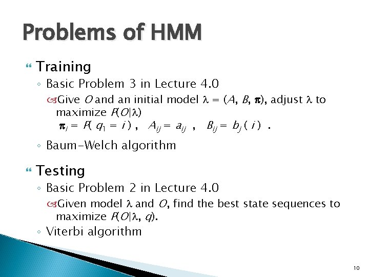
Problems of HMM Training ◦ Basic Problem 3 in Lecture 4. 0 Give O and an initial model = (A, B, ), adjust to maximize P(O| ) i = P( q 1 = i ) , Aij = aij , Bij = bj ( i ). ◦ Baum-Welch algorithm Testing ◦ Basic Problem 2 in Lecture 4. 0 Given model and O, find the best state sequences to maximize P(O| , q). ◦ Viterbi algorithm 10

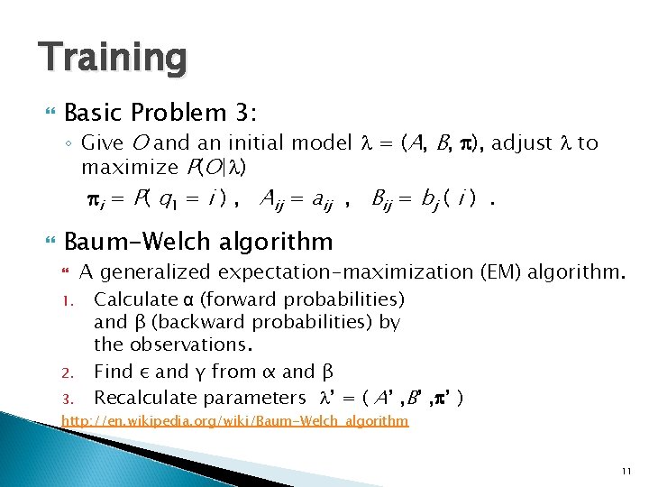
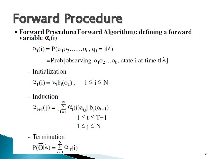
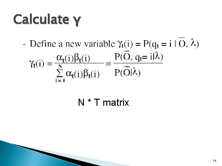
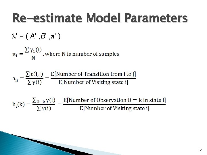
Training Basic Problem 3: ◦ Give O and an initial model = (A, B, ), adjust to maximize P(O| ) i = P( q 1 = i ) , Aij = aij , Bij = bj ( i ). Baum-Welch algorithm A generalized expectation-maximization (EM) algorithm. 1. Calculate α (forward probabilities) and β (backward probabilities) by the observations. 2. Find ε and γ from α and β 3. Recalculate parameters ’ = ( A’ , B’ , ’ ) http: //en. wikipedia. org/wiki/Baum-Welch_algorithm 11

Forward Procedure 12

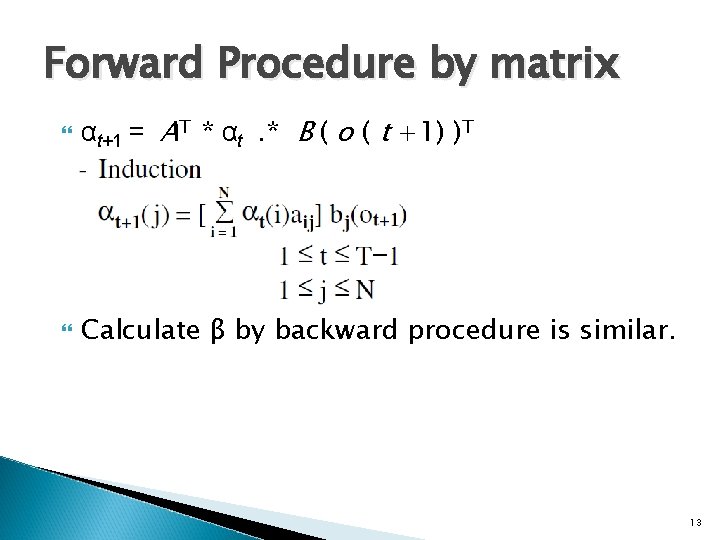
Forward Procedure by matrix αt+1 = AT * αt. * B ( o ( t +1) )T Calculate β by backward procedure is similar. 13

Calculate γ N * T matrix 14

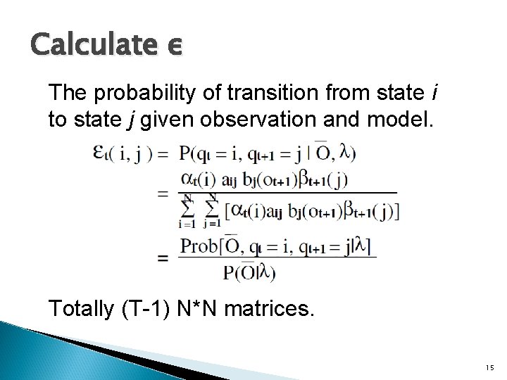
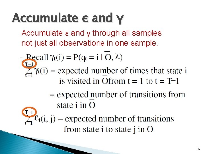
Calculate ε The probability of transition from state i to state j given observation and model. Totally (T-1) N*N matrices. 15

Accumulate ε and γ through all samples not just all observations in one sample. 16

Re-estimate Model Parameters ’ = ( A’ , B’ , ’ ) 17

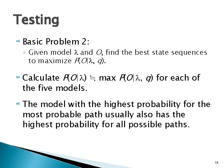
Testing Basic Problem 2: ◦ Given model and O, find the best state sequences to maximize P(O| , q). Calculate P(O| ) ≒ max P(O| , q) for each of the five models. The model with the highest probability for the most probable path usually also has the highest probability for all possible paths. 18

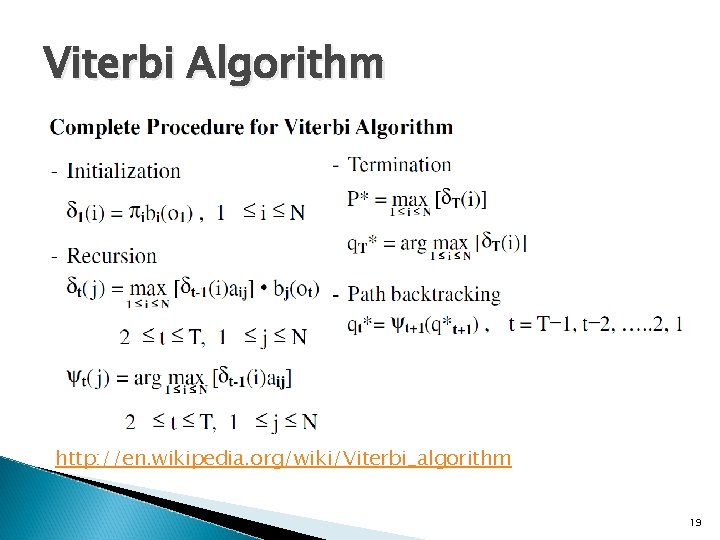
Viterbi Algorithm http: //en. wikipedia. org/wiki/Viterbi_algorithm 19

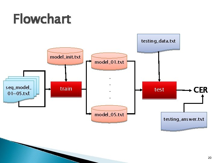
Flowchart testing_data. txt model_init. txt seq_model_ 01~05. txt train model_01. txt . . model_05. txt test CER testing_answer. txt 20

File Format 21

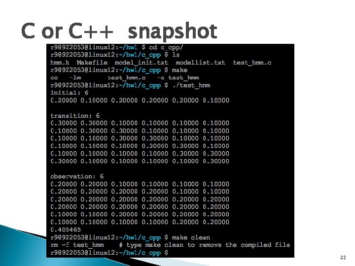
C or C++ snapshot 22

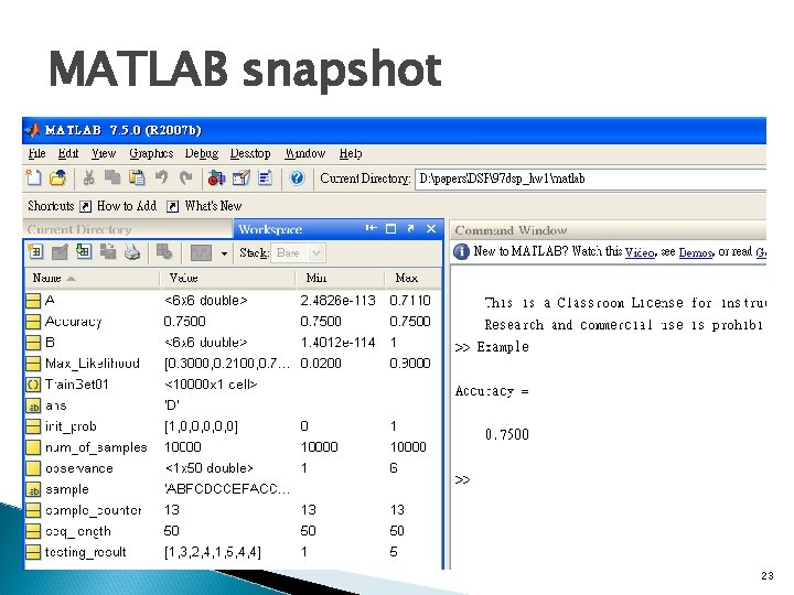
MATLAB snapshot 23

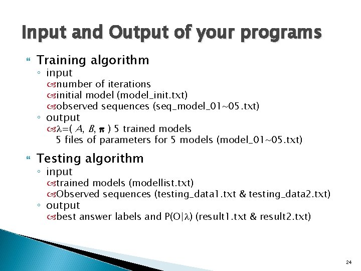
Input and Output of your programs Training algorithm ◦ input number of iterations initial model (model_init. txt) observed sequences (seq_model_01~05. txt) ◦ output =( A, B, ) 5 trained models 5 files of parameters for 5 models (model_01~05. txt) Testing algorithm ◦ input trained models (modellist. txt) Observed sequences (testing_data 1. txt & testing_data 2. txt) ◦ output best answer labels and P(O| ) (result 1. txt & result 2. txt) 24

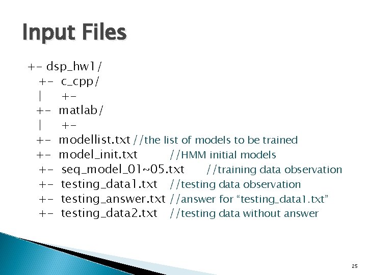
Input Files +- dsp_hw 1/ +- c_cpp/ | ++- matlab/ | ++- modellist. txt //the list of models to be trained +- model_init. txt //HMM initial models +- seq_model_01~05. txt //training data observation +- testing_data 1. txt //testing data observation +- testing_answer. txt //answer for “testing_data 1. txt” +- testing_data 2. txt //testing data without answer 25

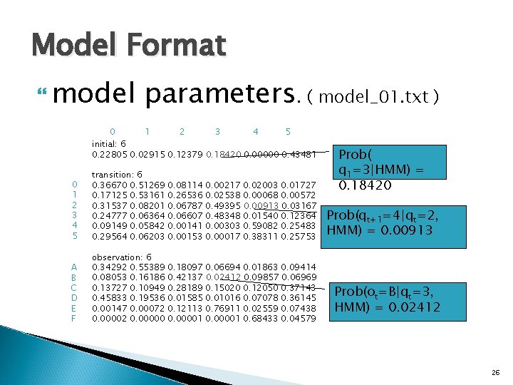
Model Format model parameters. ( model_01. txt ) 0 1 2 3 4 5 initial: 6 0. 22805 0. 02915 0. 12379 0. 18420 0. 00000 0. 43481 0 1 2 3 4 5 transition: 6 0. 36670 0. 51269 0. 17125 0. 53161 0. 31537 0. 08201 0. 24777 0. 06364 0. 09149 0. 05842 0. 29564 0. 06203 0. 08114 0. 26536 0. 06787 0. 06607 0. 00141 0. 00153 0. 00217 0. 02538 0. 49395 0. 48348 0. 00303 0. 00017 A B C D E F observation: 6 0. 34292 0. 55389 0. 08053 0. 16186 0. 13727 0. 10949 0. 45833 0. 19536 0. 00147 0. 00072 0. 00000 0. 18097 0. 42137 0. 28189 0. 01585 0. 12113 0. 00001 0. 06694 0. 01863 0. 09414 0. 02412 0. 09857 0. 06969 0. 15020 0. 12050 0. 37143 0. 01016 0. 07078 0. 36145 0. 76911 0. 02559 0. 07438 0. 00001 0. 68433 0. 04579 0. 02003 0. 01727 0. 00068 0. 00572 0. 00913 0. 03167 0. 01540 0. 12364 0. 59082 0. 25483 0. 38311 0. 25753 Prob( q 1=3|HMM) = 0. 18420 Prob(qt+1=4|qt=2, HMM) = 0. 00913 Prob(ot=B|qt=3, HMM) = 0. 02412 26

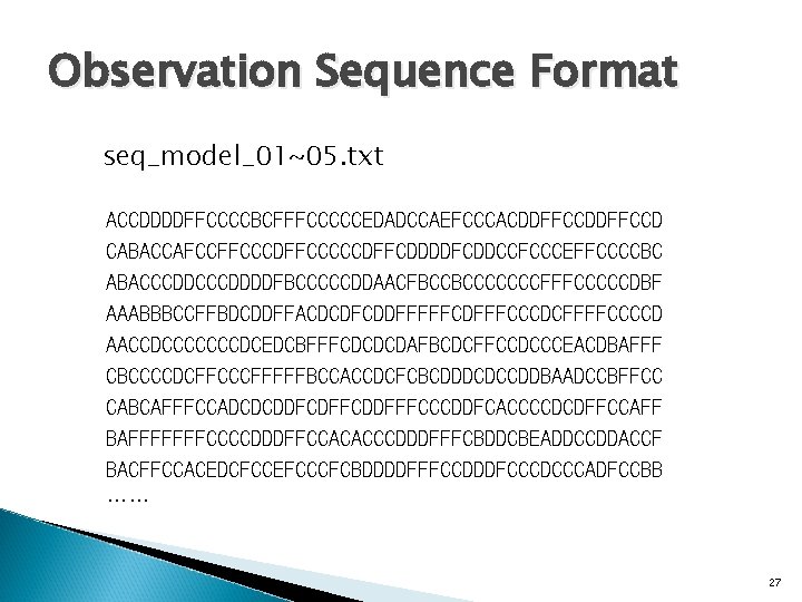
Observation Sequence Format seq_model_01~05. txt ACCDDDDFFCCCCBCFFFCCCCCEDADCCAEFCCCACDDFFCCD CABACCAFCCFFCCCDFFCCCCCDFFCDDDDFCDDCCFCCCEFFCCCCBC ABACCCDDDDFBCCCCCDDAACFBCCBCCCCCCCFFFCCCCCDBF AAABBBCCFFBDCDDFFACDCDFCDDFFFFFCDFFFCCCDCFFFFCCCCD AACCDCCCCCCCDCEDCBFFFCDCDCDAFBCDCFFCCDCCCEACDBAFFF CBCCCCDCFFCCCFFFFFBCCACCDCFCBCDDDCDCCDDBAADCCBFFCC CABCAFFFCCADCDCDDFCDFFCDDFFFCCCDDFCACCCCDCDFFCCAFF BAFFFFFFFCCCCDDDFFCCACACCCDDDFFFCBDDCBEADDCCDDACCF BACFFCCACEDCFCCEFCCCFCBDDDDFFFCCDDDFCCCDCCCADFCCBB …… 27

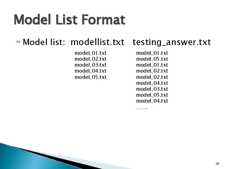
Model List Format Model list: modellist. txt testing_answer. txt model_01. txt model_02. txt model_03. txt model_04. txt model_05. txt model_01. txt model_02. txt model_04. txt model_03. txt model_05. txt model_04. txt ……. 28

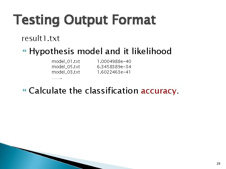
Testing Output Format result 1. txt Hypothesis model and it likelihood model_01. txt model_05. txt model_03. txt ……. 1. 0004988 e-40 6. 3458389 e-34 1. 6022463 e-41 Calculate the classification accuracy. 29

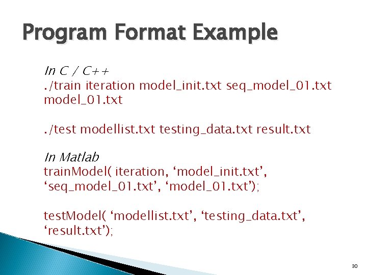
Program Format Example In C / C++ . /train iteration model_init. txt seq_model_01. txt. /test modellist. txt testing_data. txt result. txt In Matlab train. Model( iteration, ‘model_init. txt’, ‘seq_model_01. txt’, ‘model_01. txt’); test. Model( ‘modellist. txt’, ‘testing_data. txt’, ‘result. txt’); 30

Submit Requirement Send to hpttw 0608@gmail. com Subject: [DSP] HW 1 r 99 xxxxxx Your program ◦ train. c, test. c, Makefile ◦ train. Model. m, test. Model. m Your 5 Models After Training ◦ model_01~05. txt Testing result and accuracy ◦ result 1~2. txt (for testing_data 1~2. txt) ◦ acc. txt (for testing_data 1. txt) Document ( doc/pdf/html ) ◦ Name, student ID, summary of your results ◦ Specify your environment and how to execute. 31

Submit Requirement Compress your hw 1 into “hw 1_[學號]. zip” +- hw 1_[學號]/ +- train. c (train. Model. m) +- test. c (test. Model. m) +- Makefile (none for Matlab) +- model_01~05. txt +- result 1~2. txt +- acc. txt +- Document (doc/pdf/html ) 32

Contact TA hpttw 0608@gmail. com Office Hour: Tue 13: 00~14: 00 & Wed 13: 00~14: 00/電二531 Please let us know you‘re coming by email, thanks! 語音實驗室 涂宗瑋 33