EEL 6586 AUTOMATIC SPEECH PROCESSING Hidden Markov Model

EEL 6586: AUTOMATIC SPEECH PROCESSING Hidden Markov Model Lecture Mark D. Skowronski Computational Neuro-Engineering Lab University of Florida March 31, 2003

Questions to be Answered • What is a Hidden Markov Model? • How do HMMs work? • How are HMMs applied to automatic speech recognition? • What are the strengths/weaknesses of HMMs?

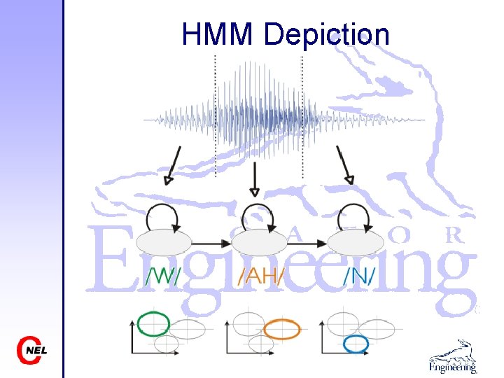
What is an HMM? A Hidden Markov Model is a piecewise stationary model of a nonstationary signal. Model parameters: • states -- represents domain of a stationary signal • interstate connections -- defines model architecture • pdf estimates (for each state) § Discrete -- codebooks § Continuous -- mean, covariance matrices

HMM Depiction

PDF Estimation • Discrete – Codebook of feature space cluster centers – Probability for each codebook entry • Continuous – Gaussian mixtures (mean, covariance, mixture weights) – Discriminative estimates (neural networks)

How do HMMs Work? • Three fundamental issues – Training: Baum-Welch algorithm – Scoring (evaluation): Forward algorithm – Optimal path: Viterbi algorithm Complete implementation details: “A Tutorial on Hidden Markov Models and Selected Applications in Speech Recognition”, L. R. Rabiner, IEEE Proceedings, Feb 1989

HMM Training • Baum-Welch algorithm – Iterative procedure (on-line or batch mode) – Guaranteed to increase model accuracy after each iteration – Estimation may be model-based (ML) or discriminative (MMI)

HMM Evaluation • Forward algorithm – Calculates P(O|λ) for ALL valid state sequences – Complexity: • order N 2 T, ~5000 computations • order 2 T • NT (brute force), ~6 E 86 computations • N states, T speech frames

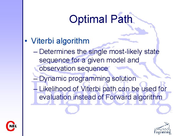
Optimal Path • Viterbi algorithm – Determines the single most-likely state sequence for a given model and observation sequence – Dynamic programming solution – Likelihood of Viterbi path can be used for evaluation instead of Forward algorithm

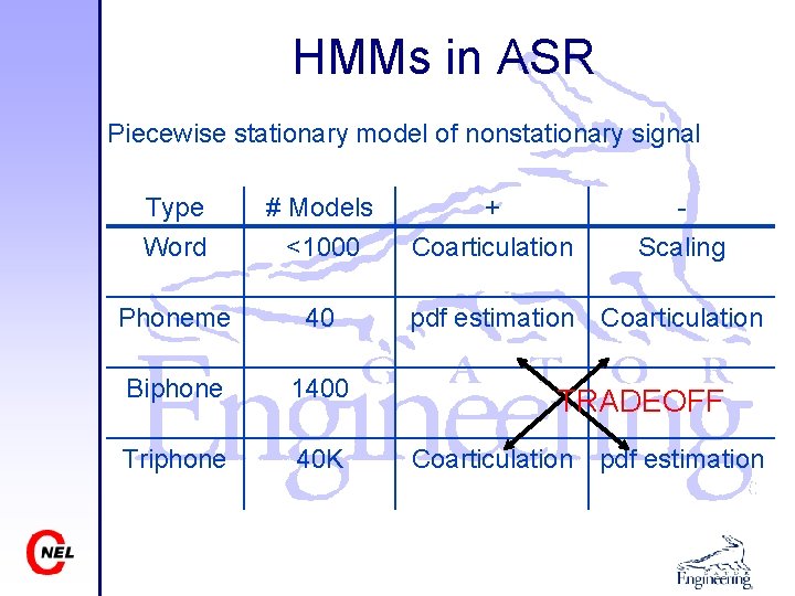
HMMs in ASR Piecewise stationary model of nonstationary signal Type Word # Models <1000 Phoneme 40 Biphone 1400 Triphone 40 K + Coarticulation Scaling pdf estimation Coarticulation TRADEOFF Coarticulation pdf estimation

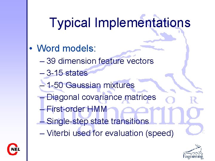
Typical Implementations • Word models: – 39 dimension feature vectors – 3 -15 states – 1 -50 Gaussian mixtures – Diagonal covariance matrices – First-order HMM – Single-step state transitions – Viterbi used for evaluation (speed)

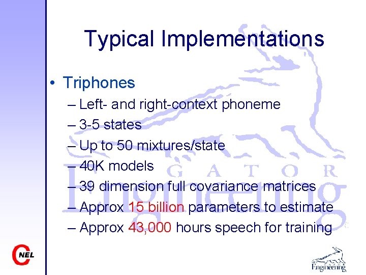
Typical Implementations • Triphones – Left- and right-context phoneme – 3 -5 states – Up to 50 mixtures/state – 40 K models – 39 dimension full covariance matrices – Approx 15 billion parameters to estimate – Approx 43, 000 hours speech for training

Implementation Issues • Same number of states for each word model? • Underflow of evaluation probabilities? • Full/Diagonal covariance matrices?

HMM Limitations • Piecewise stationary assumption – Dipthongs – Tonal languages – Phonetic information in transitions • iid assumption – Slow articulators • Temporal information – No modeling beyond 100 ms time frame • Data intensive

Download Slides www. cnel. ufl. edu/~markskow/papers/hmm. ppt