Digital Image Processing Chapter 10 Image Description and

Digital Image Processing Chapter 10: Image Description and Representation 5 September 2013

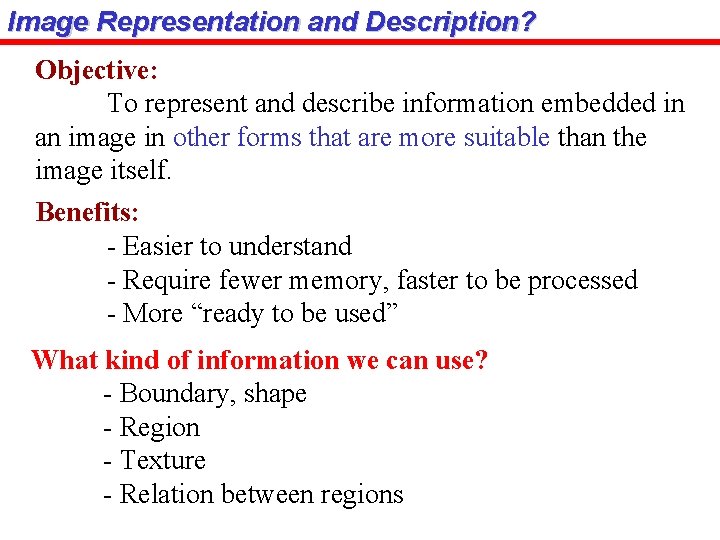
Image Representation and Description? Objective: To represent and describe information embedded in an image in other forms that are more suitable than the image itself. Benefits: - Easier to understand - Require fewer memory, faster to be processed - More “ready to be used” What kind of information we can use? - Boundary, shape - Region - Texture - Relation between regions

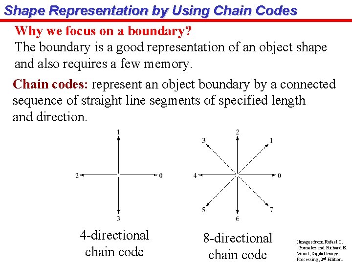
Shape Representation by Using Chain Codes Why we focus on a boundary? The boundary is a good representation of an object shape and also requires a few memory. Chain codes: represent an object boundary by a connected sequence of straight line segments of specified length and direction. 4 -directional chain code 8 -directional chain code (Images from Rafael C. Gonzalez and Richard E. Wood, Digital Image Processing, 2 nd Edition.

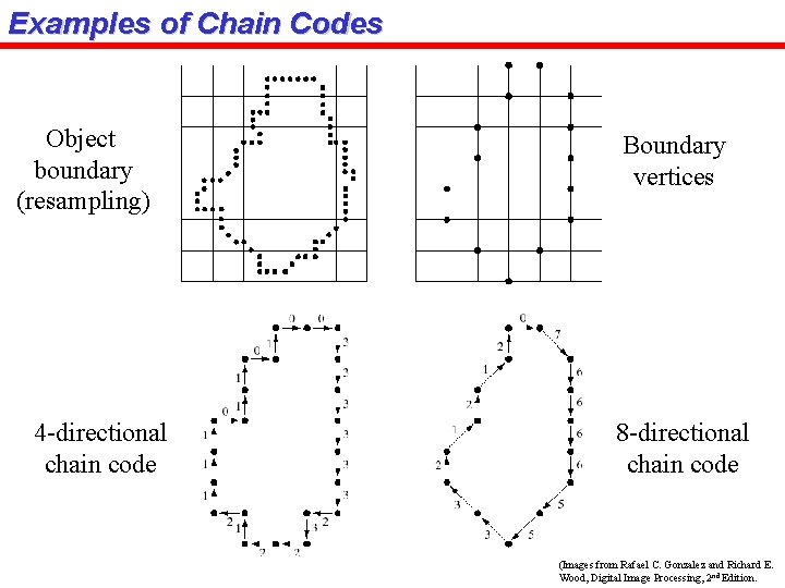
Examples of Chain Codes Object boundary (resampling) 4 -directional chain code Boundary vertices 8 -directional chain code (Images from Rafael C. Gonzalez and Richard E. Wood, Digital Image Processing, 2 nd Edition.

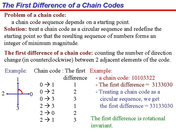
The First Difference of a Chain Codes Problem of a chain code: a chain code sequence depends on a starting point. Solution: treat a chain code as a circular sequence and redefine the starting point so that the resulting sequence of numbers forms an integer of minimum magnitude. The first difference of a chain code: counting the number of direction change (in counterclockwise) between 2 adjacent elements of the code. Example: 1 2 3 Chain code : The first Example: difference - a chain code: 10103322 0 1 1 - The first difference = 3133030 2 - Treating a chain code as a 0 0 2 0 3 3 circular sequence, we get 2 3 1 the first difference = 33133030 2 The first difference is rotational 2 1 3 invariant.

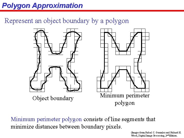
Polygon Approximation Represent an object boundary by a polygon Object boundary Minimum perimeter polygon consists of line segments that minimize distances between boundary pixels. (Images from Rafael C. Gonzalez and Richard E. Wood, Digital Image Processing, 2 nd Edition.

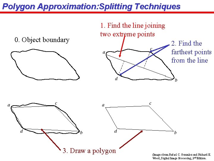
Polygon Approximation: Splitting Techniques 0. Object boundary 1. Find the line joining two extreme points 3. Draw a polygon 2. Find the farthest points from the line (Images from Rafael C. Gonzalez and Richard E. Wood, Digital Image Processing, 2 nd Edition.

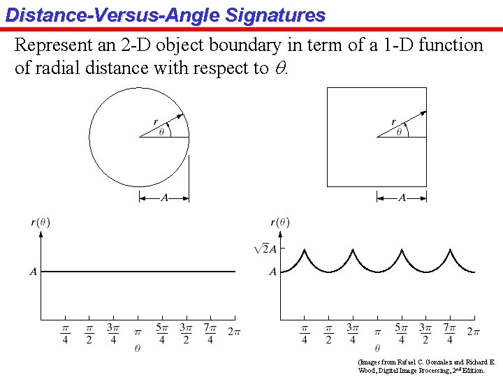
Distance-Versus-Angle Signatures Represent an 2 -D object boundary in term of a 1 -D function of radial distance with respect to q. (Images from Rafael C. Gonzalez and Richard E. Wood, Digital Image Processing, 2 nd Edition.

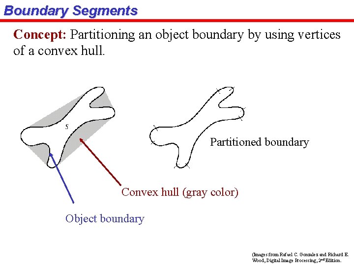
Boundary Segments Concept: Partitioning an object boundary by using vertices of a convex hull. Partitioned boundary Convex hull (gray color) Object boundary (Images from Rafael C. Gonzalez and Richard E. Wood, Digital Image Processing, 2 nd Edition.

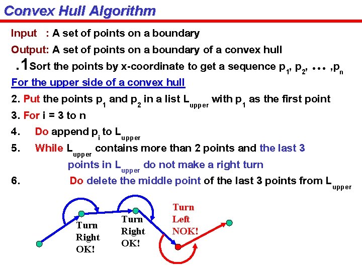
Convex Hull Algorithm Input : A set of points on a boundary Output: A set of points on a boundary of a convex hull. 1 Sort the points by x-coordinate to get a sequence p 1, p 2, … , pn For the upper side of a convex hull 2. Put the points p 1 and p 2 in a list Lupper with p 1 as the first point 3. For i = 3 to n 4. Do append pi to Lupper 5. While Lupper contains more than 2 points and the last 3 points in Lupper do not make a right turn 6. Do delete the middle point of the last 3 points from Lupper Turn Right OK! Turn Left NOK!

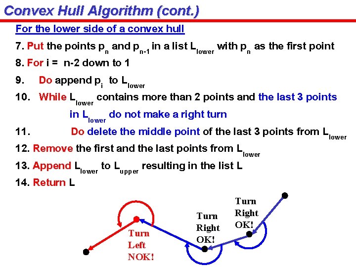
Convex Hull Algorithm (cont. ) For the lower side of a convex hull 7. Put the points pn and pn-1 in a list Llower with pn as the first point 8. For i = n-2 down to 1 9. Do append pi to Llower 10. While Llower contains more than 2 points and the last 3 points in Llower do not make a right turn 11. Do delete the middle point of the last 3 points from Llower 12. Remove the first and the last points from Llower 13. Append Llower to Lupper resulting in the list L 14. Return L Turn Left NOK! Turn Right OK!

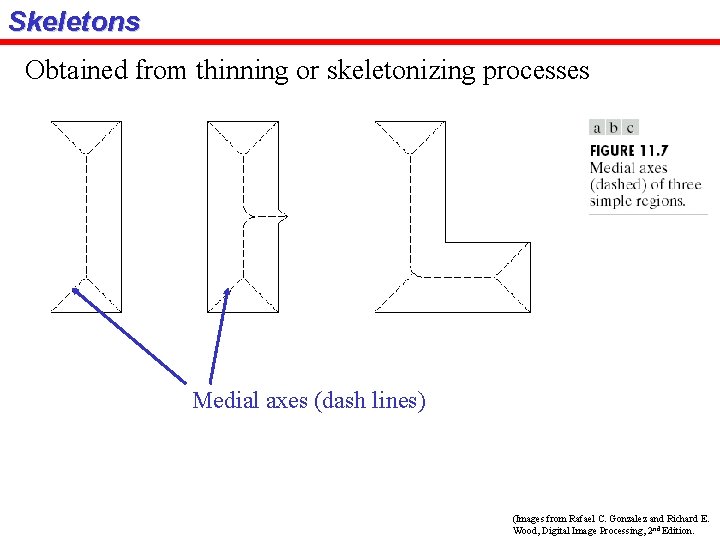
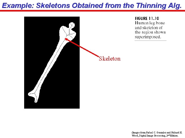
Skeletons Obtained from thinning or skeletonizing processes Medial axes (dash lines) (Images from Rafael C. Gonzalez and Richard E. Wood, Digital Image Processing, 2 nd Edition.

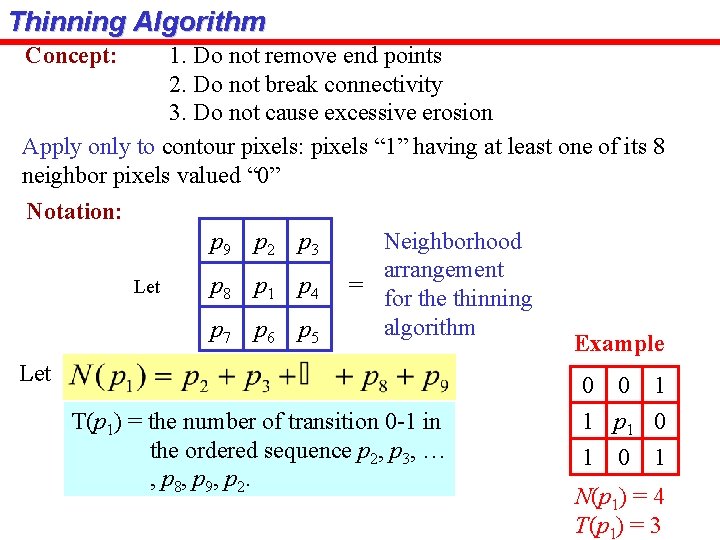
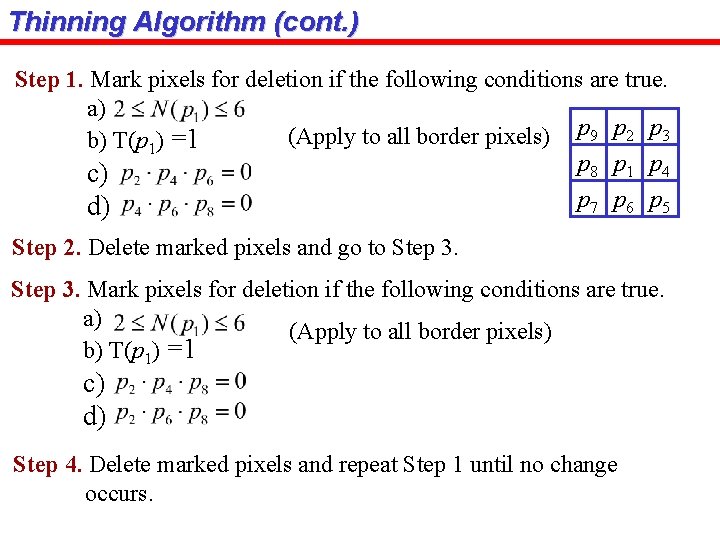
Thinning Algorithm Concept: 1. Do not remove end points 2. Do not break connectivity 3. Do not cause excessive erosion Apply only to contour pixels: pixels “ 1” having at least one of its 8 neighbor pixels valued “ 0” Notation: Neighborhood p 9 p 2 p 3 arrangement p 8 p 1 p 4 = Let for the thinning algorithm p 7 p 6 p 5 Example Let 0 0 1 T(p 1) = the number of transition 0 -1 in the ordered sequence p 2, p 3, … , p 8, p 9, p 2. 1 p 1 0 1 N(p 1) = 4 T(p 1) = 3

Thinning Algorithm (cont. ) Step 1. Mark pixels for deletion if the following conditions are true. a) p 9 p 2 p 3 (Apply to all border pixels) b) T(p 1) =1 p 8 p 1 p 4 c) p 7 p 6 p 5 d) Step 2. Delete marked pixels and go to Step 3. Mark pixels for deletion if the following conditions are true. a) (Apply to all border pixels) b) T(p 1) =1 c) d) Step 4. Delete marked pixels and repeat Step 1 until no change occurs.

Example: Skeletons Obtained from the Thinning Alg. Skeleton (Images from Rafael C. Gonzalez and Richard E. Wood, Digital Image Processing, 2 nd Edition.

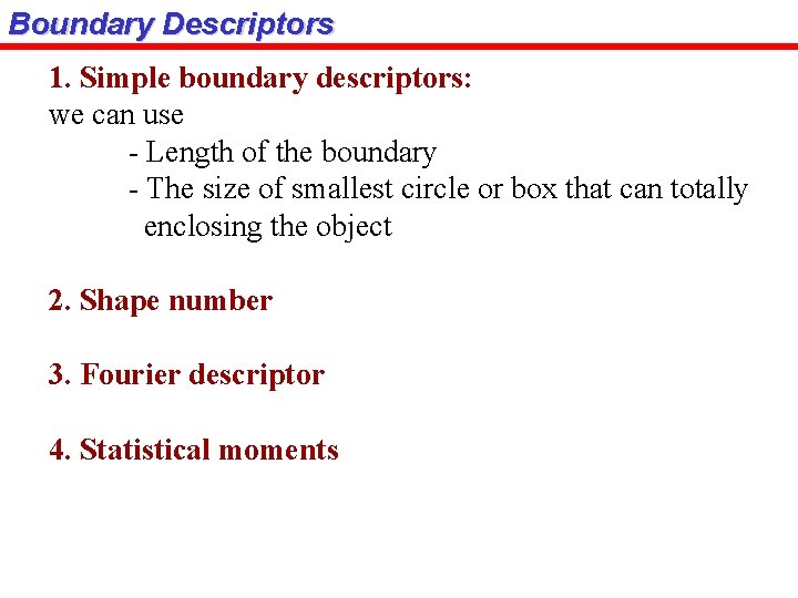
Boundary Descriptors 1. Simple boundary descriptors: we can use - Length of the boundary - The size of smallest circle or box that can totally enclosing the object 2. Shape number 3. Fourier descriptor 4. Statistical moments

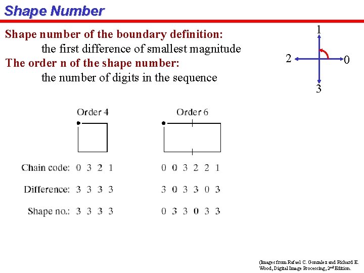
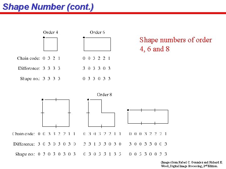
Shape Number Shape number of the boundary definition: the first difference of smallest magnitude The order n of the shape number: the number of digits in the sequence 1 2 0 3 (Images from Rafael C. Gonzalez and Richard E. Wood, Digital Image Processing, 2 nd Edition.

Shape Number (cont. ) Shape numbers of order 4, 6 and 8 (Images from Rafael C. Gonzalez and Richard E. Wood, Digital Image Processing, 2 nd Edition.

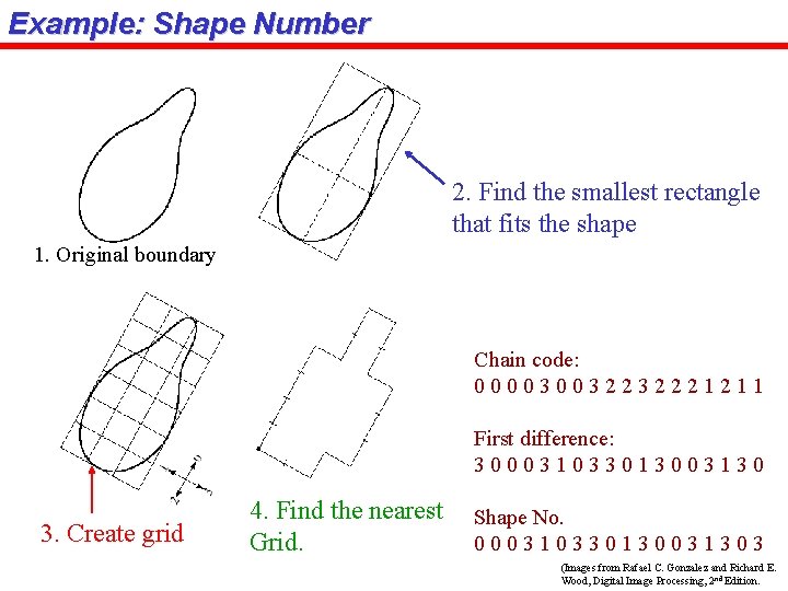
Example: Shape Number 2. Find the smallest rectangle that fits the shape 1. Original boundary Chain code: 000030032232221211 First difference: 300031033013003130 3. Create grid 4. Find the nearest Grid. Shape No. 000310330130031303 (Images from Rafael C. Gonzalez and Richard E. Wood, Digital Image Processing, 2 nd Edition.

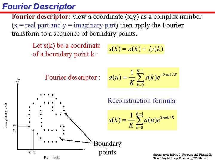
Fourier Descriptor Fourier descriptor: view a coordinate (x, y) as a complex number (x = real part and y = imaginary part) then apply the Fourier transform to a sequence of boundary points. Let s(k) be a coordinate of a boundary point k : Fourier descriptor : Reconstruction formula Boundary points (Images from Rafael C. Gonzalez and Richard E. Wood, Digital Image Processing, 2 nd Edition.

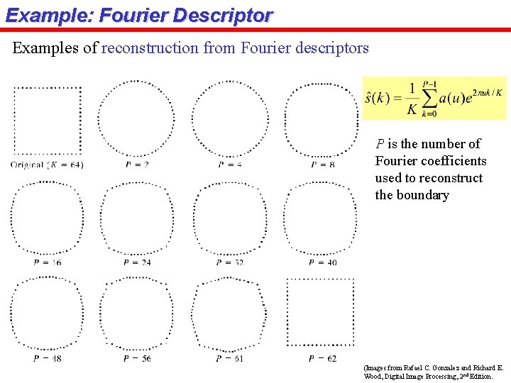
Example: Fourier Descriptor Examples of reconstruction from Fourier descriptors P is the number of Fourier coefficients used to reconstruct the boundary (Images from Rafael C. Gonzalez and Richard E. Wood, Digital Image Processing, 2 nd Edition.

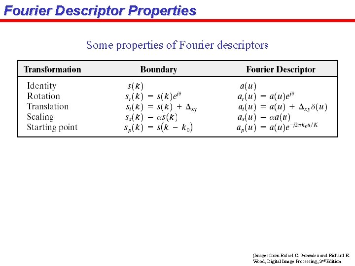
Fourier Descriptor Properties Some properties of Fourier descriptors (Images from Rafael C. Gonzalez and Richard E. Wood, Digital Image Processing, 2 nd Edition.

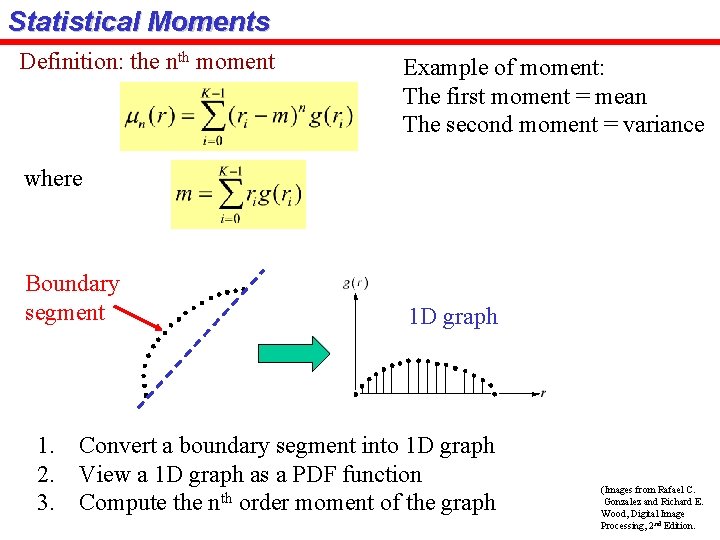
Statistical Moments Definition: the nth moment Example of moment: The first moment = mean The second moment = variance where Boundary segment 1 D graph 1. Convert a boundary segment into 1 D graph 2. View a 1 D graph as a PDF function 3. Compute the nth order moment of the graph (Images from Rafael C. Gonzalez and Richard E. Wood, Digital Image Processing, 2 nd Edition.

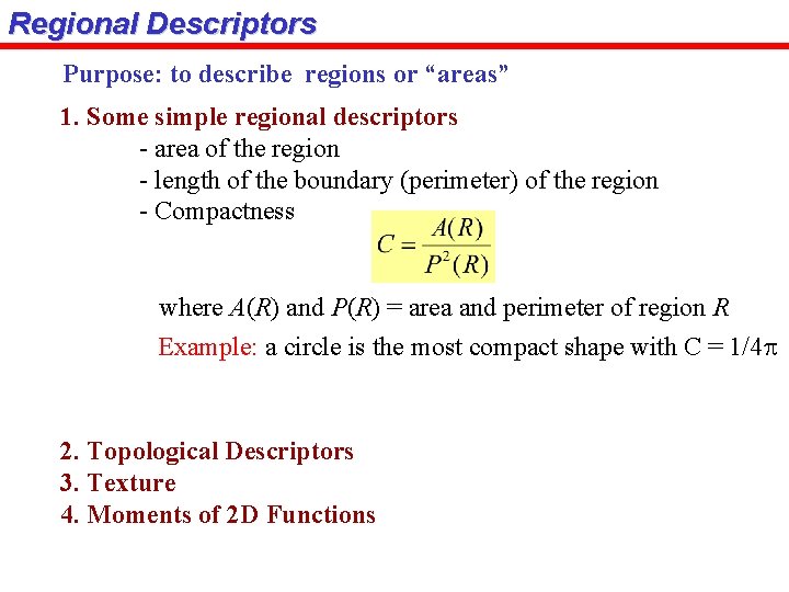
Regional Descriptors Purpose: to describe regions or “areas” 1. Some simple regional descriptors - area of the region - length of the boundary (perimeter) of the region - Compactness where A(R) and P(R) = area and perimeter of region R Example: a circle is the most compact shape with C = 1/4 p 2. Topological Descriptors 3. Texture 4. Moments of 2 D Functions

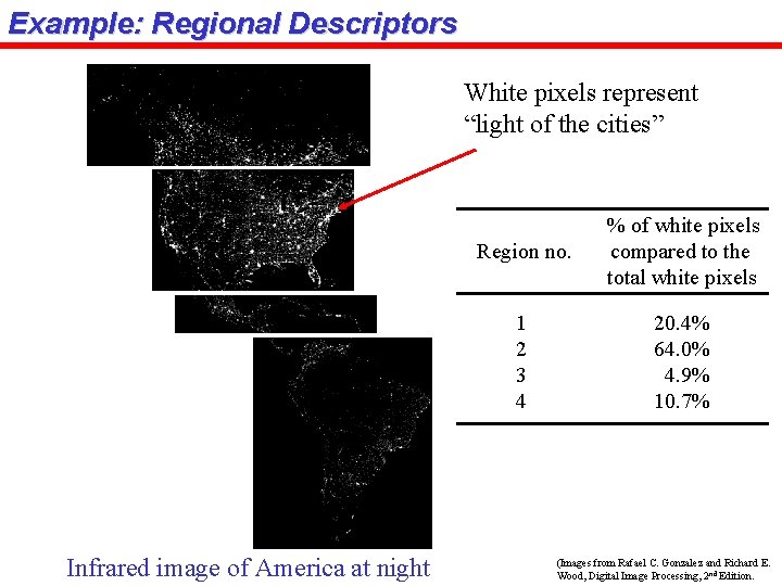
Example: Regional Descriptors White pixels represent “light of the cities” Infrared image of America at night Region no. % of white pixels compared to the total white pixels 1 2 3 4 20. 4% 64. 0% 4. 9% 10. 7% (Images from Rafael C. Gonzalez and Richard E. Wood, Digital Image Processing, 2 nd Edition.

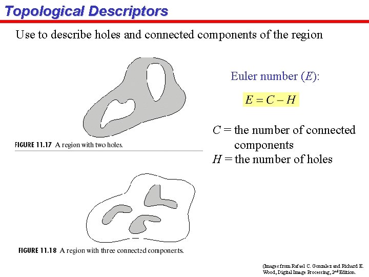
Topological Descriptors Use to describe holes and connected components of the region Euler number (E): C = the number of connected components H = the number of holes (Images from Rafael C. Gonzalez and Richard E. Wood, Digital Image Processing, 2 nd Edition.

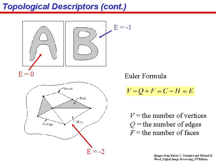
Topological Descriptors (cont. ) E = -1 E=0 Euler Formula V = the number of vertices Q = the number of edges F = the number of faces E = -2 (Images from Rafael C. Gonzalez and Richard E. Wood, Digital Image Processing, 2 nd Edition.

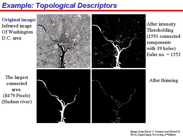
Example: Topological Descriptors Original image: Infrared image Of Washington D. C. area The largest connected area (8479 Pixels) (Hudson river) After intensity Thresholding (1591 connected components with 39 holes) Euler no. = 1552 After thinning (Images from Rafael C. Gonzalez and Richard E. Wood, Digital Image Processing, 2 nd Edition.

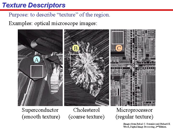
Texture Descriptors Purpose: to describe “texture” of the region. Examples: optical microscope images: B C A Superconductor (smooth texture) Cholesterol (coarse texture) Microprocessor (regular texture) (Images from Rafael C. Gonzalez and Richard E. Wood, Digital Image Processing, 2 nd Edition.

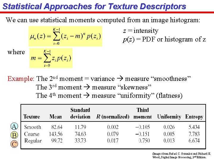
Statistical Approaches for Texture Descriptors We can use statistical moments computed from an image histogram: z = intensity p(z) = PDF or histogram of z where Example: The 2 nd moment = variance measure “smoothness” The 3 rd moment measure “skewness” The 4 th moment measure “uniformity” (flatness) A B C (Images from Rafael C. Gonzalez and Richard E. Wood, Digital Image Processing, 2 nd Edition.

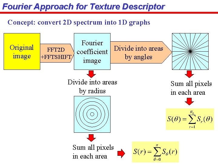
Fourier Approach for Texture Descriptor Concept: convert 2 D spectrum into 1 D graphs Fourier Original FFT 2 D coefficient Divide into areas image +FFTSHIFT by angles image Divide into areas by radius Sum all pixels in each area

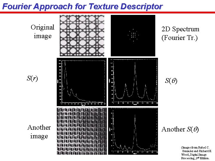
Fourier Approach for Texture Descriptor Original image S(r) Another image 2 D Spectrum (Fourier Tr. ) S(q) Another S(q) (Images from Rafael C. Gonzalez and Richard E. Wood, Digital Image Processing, 2 nd Edition.

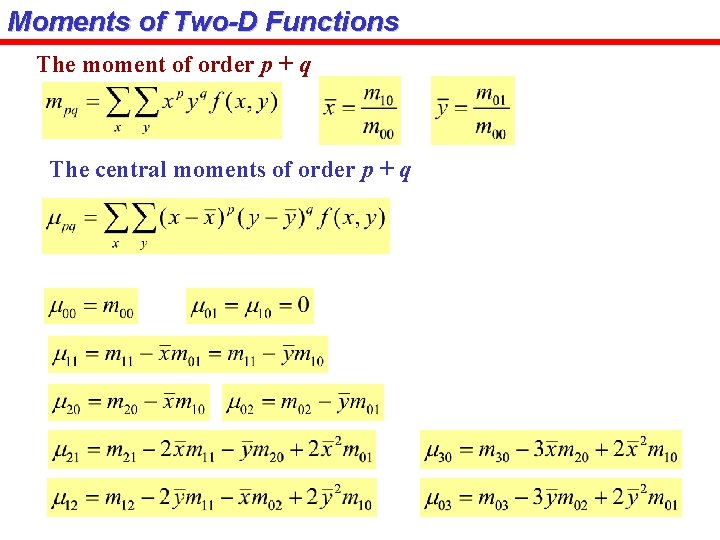
Moments of Two-D Functions The moment of order p + q The central moments of order p + q

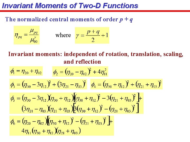
Invariant Moments of Two-D Functions The normalized central moments of order p + q where Invariant moments: independent of rotation, translation, scaling, and reflection

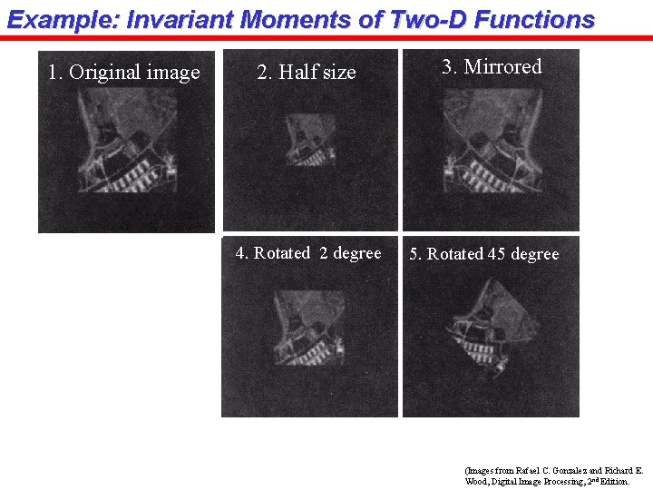
Example: Invariant Moments of Two-D Functions 1. Original image 2. Half size 4. Rotated 2 degree 3. Mirrored 5. Rotated 45 degree (Images from Rafael C. Gonzalez and Richard E. Wood, Digital Image Processing, 2 nd Edition.

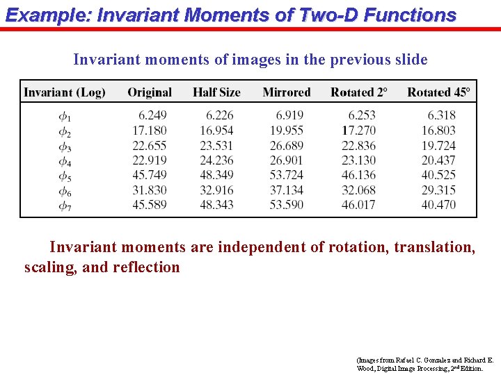
Example: Invariant Moments of Two-D Functions Invariant moments of images in the previous slide Invariant moments are independent of rotation, translation, scaling, and reflection (Images from Rafael C. Gonzalez and Richard E. Wood, Digital Image Processing, 2 nd Edition.

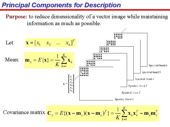
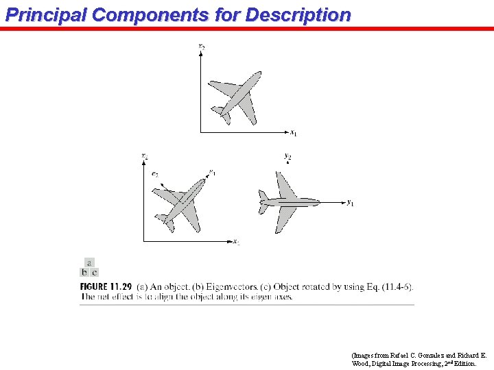
Principal Components for Description Purpose: to reduce dimensionality of a vector image while maintaining information as much as possible. Let Mean: Covariance matrix

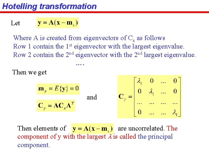
Hotelling transformation Let Where A is created from eigenvectors of Cx as follows Row 1 contain the 1 st eigenvector with the largest eigenvalue. Row 2 contain the 2 nd eigenvector with the 2 nd largest eigenvalue. …. Then we get and Then elements of are uncorrelated. The component of y with the largest l is called the principal component.

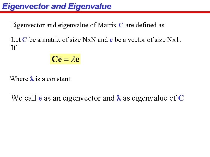
Eigenvector and Eigenvalue Eigenvector and eigenvalue of Matrix C are defined as Let C be a matrix of size Nx. N and e be a vector of size Nx 1. If Where l is a constant We call e as an eigenvector and l as eigenvalue of C

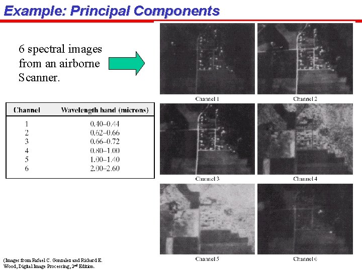
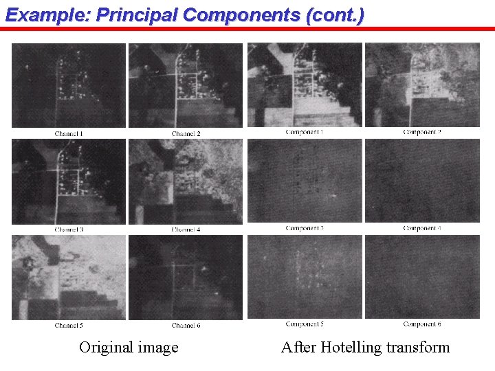
Example: Principal Components 6 spectral images from an airborne Scanner. (Images from Rafael C. Gonzalez and Richard E. Wood, Digital Image Processing, 2 nd Edition.

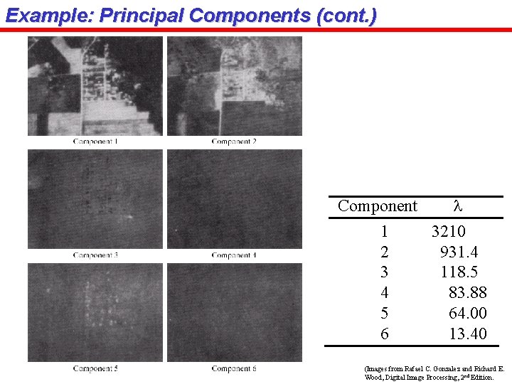
Example: Principal Components (cont. ) Component l 1 3210 2 931. 4 3 118. 5 4 83. 88 5 64. 00 6 13. 40 (Images from Rafael C. Gonzalez and Richard E. Wood, Digital Image Processing, 2 nd Edition.

Example: Principal Components (cont. ) Original image After Hotelling transform

Principal Components for Description (Images from Rafael C. Gonzalez and Richard E. Wood, Digital Image Processing, 2 nd Edition.