Determine whether the function is continuous at x

Determine whether the function is continuous at x = 2. A. yes B. no

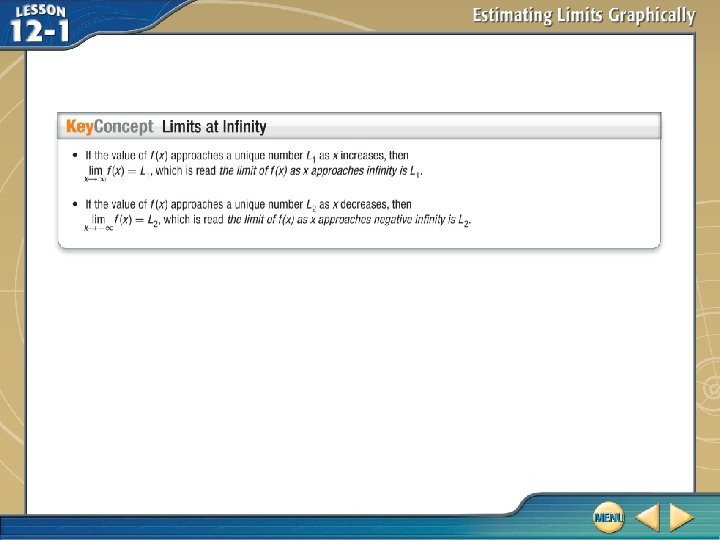
You estimated limits to determine the continuity and end behavior of functions. (Lesson 1 -3) • Estimate limits of functions at fixed values. • Estimate limits of functions at infinity.

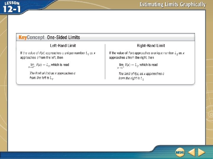
• one-sided limit • two-sided limit

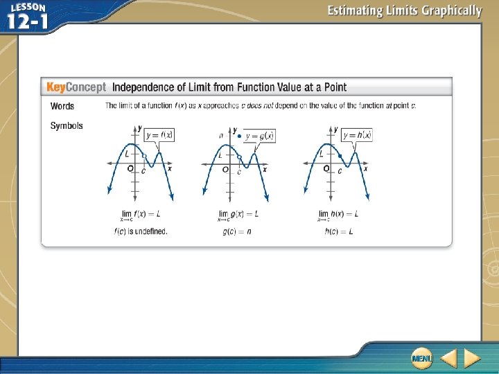
Estimate a Limit = f (c) Estimate using a graph. Support your conjecture using a table of values. Analyze Graphically The graph of f (x) = 4 x + 1 suggests that as x gets closer to – 7, the corresponding function values get closer to – 27. Therefore, we can estimate that = – 27.

Estimate a Limit = f (c) Support Numerically Make a table of values for f, choosing x-values that approach – 7 by using some values slightly less than – 7 and some values slightly greater than – 7.

Estimate a Limit = f (c) The pattern of outputs suggests that as x gets close to – 7 from the left or right, f (x) gets closer to – 27. This supports our graphical analysis. Answer: – 27

Estimate using a graph. A. 3, C. – 1, B. 1, D. – 3,

Estimate a Limit ≠ f (c) Estimate using a graph. Support your conjecture using a table of values. Analyze Graphically The graph of suggests that as x gets closer to 4, the corresponding function value approaches 8. Therefore, we can estimate that is 8.

Estimate a Limit ≠ f (c) Support Numerically Make a table of values, choosing x-values that approach 4 from either side.

Estimate a Limit ≠ f (c) The pattern of outputs suggests that as x gets closer to 4, f (x) gets closer to 8. This supports our graphical analysis. Answer: 8

Estimate using a graph. A. 0, C. 6, B. 0, D. – 6,

Estimate One-Sided and Two-Sided Limits A. Estimate each one-sided or two-sided limit, if it exists. The graph of suggests that f (x) = – 2 and f (x) = 3. Because the left- and right-hand limits of f (x) as x approaches 1 are not the same, does not exist.

Estimate One-Sided and Two-Sided Limits Answer:

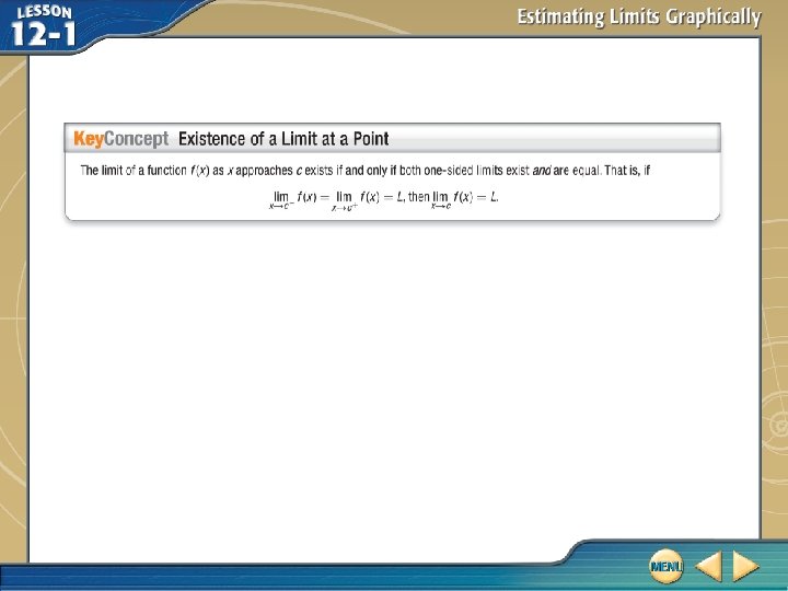
Estimate One-Sided and Two-Sided Limits B. Estimate each one-sided or two-sided limit, if it exists. 0 0 The graph of g(x) suggests that g(x) = – 1 and g(x) = – 1. Because the left- and right-hand limits of g(x) as x approaches 0 are the same, and is – 1. exists

Estimate One-Sided and Two-Sided Limits Answer:

Estimate each one-sided or two-sided limit, if it exists. A. B. C. D.

Limits and Unbounded Behavior A. Estimate , if it exists. Analyze Graphically The graph of and suggests that because as x gets closer to 2, the function values of the graph increase.

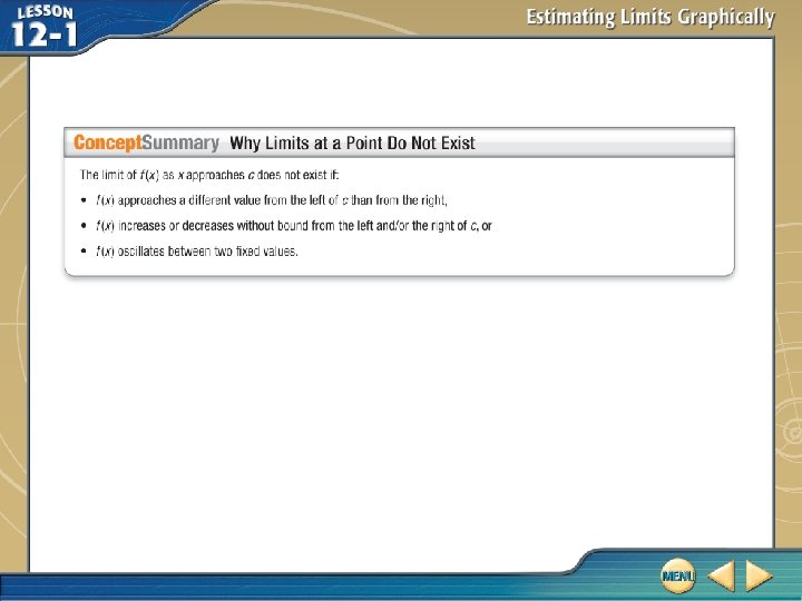
Limits and Unbounded Behavior Neither one-sided limit at x = 2 exists; therefore, we can conclude that does not exist. However, because both sides approach ∞, we describe the behavior of f(x) at 2 by writing Support Numerically .

Limits and Unbounded Behavior The pattern of outputs suggests that as x gets closer to 2 from the left and the right, f(x) grows without bound. This supports our graphical analysis. Answer: ∞

Limits and Unbounded Behavior B. Estimate , if it exists. Analyze Graphically The graph of and suggests that because as x gets closer to 0, the function values from the left decrease and the function values from the right increase.

Limits and Unbounded Behavior Neither one-sided limit at x = 0 exists; therefore, does not exist. In this case, we cannot describe the behavior of f(x) at 0 using a single expression because the unbounded behaviors from the left and right differ. Support Numerically

Limits and Unbounded Behavior The pattern of outputs suggests that as x gets closer to 0 from the left and the right, f(x) decreases and increases without bound, respectively. This supports our graphical analysis. Answer: does not exist

Use a graph to estimate , if it exists. A. ∞, C. ∞, B. –∞, D. –∞,

Limits and Oscillating Behavior Estimate , if it exists. The graph of f(x) = x sin x suggests that as x gets closer to 0, the corresponding function values get closer and closer to 0.

Limits and Oscillating Behavior Therefore, Answer: 0 .

Estimate A. does not exist B. 1 C. 0 D. – 1 , if it exists.

Estimate Limits at Infinity A. Estimate , if it exists. Analyze Graphically The graph of suggests that As x increases, f(x) gets closer to 1. .

Estimate Limits at Infinity Support Numerically The pattern of outputs suggests that as x increases, f(x) approaches 1. Answer: 1

Estimate Limits at Infinity B. Estimate , if it exists. Analyze Graphically The graph of suggests that = – 1. As x increases, f(x) gets closer to – 1.

Estimate Limits at Infinity Support Numerically The pattern of outputs suggests that as x increases, f(x) approaches – 1. Answer: – 1

Estimate Limits at Infinity C. Estimate , if it exists. Analyze Graphically The graph of f(x) = cos x suggests that does not exist. As x increases, f(x) oscillates between 1 and – 1.

Estimate Limits at Infinity Support Numerically The pattern of outputs suggests that as x increases, f(x) oscillates between 1 and – 1. Answer: does not exist

Estimate A. – 2 B. 2 C. –∞ D. ∞ , if it exists.

Estimate Limits at Infinity A. BACTERIA The growth of a certain bacteria can be modeled by the logistic growth function , where t represents time in hours. Estimate result. , if it exists, and interpret your

Estimate Limits at Infinity Graph using a graphing calculator. The graph shows that when t = 20, B(t) ≈ 674. 44. Notice that as t increases, the function values of the graph get closer and closer to 675. So we can estimate that .

Estimate Limits at Infinity B. POPULATION The population growth of a certain city is given by the function P(t) = 0. 7(1. 1)t, where t is time in years. Estimate , if it exists, and interpret your result. Graph the function P(t ) = 0. 7(1. 1)t using a graphing calculator. The graph shows that as t increases the function values increase. So, we can estimate that.

Estimate Limits at Infinity Interpret the Result If the pattern continues, the population will grow without bound over time. Answer: ; If the pattern continues, the population will grow without bound over time.

POPULATION The population growth of deer on Fawn Island is given by P (t) = 200(0. 81)t, where t is time given in years. Estimate , if it exists, and interpret your results. A. ; Over time, the deer population will grow without bound. B. ; Over time, the deer population will reach 0. C. ; Over time, the deer population will reach 200. D. ; Over time, the deer population will reach 162.

• one-sided limit • two-sided limit