CSE 245 Computer Aided Circuit Simulation and Verification

CSE 245: Computer Aided Circuit Simulation and Verification Matrix Computations: Iterative Methods (II) Chung-Kuan Cheng

Outline o Introduction o Direct Methods o Iterative Methods n n n Formulations Projection Methods Krylov Space Methods Preconditioned Iterations Multigrid Methods Domain Decomposition Methods 2

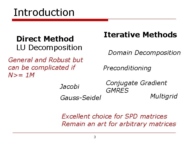
Introduction Iterative Methods Direct Method LU Decomposition Domain Decomposition General and Robust but can be complicated if N>= 1 M Preconditioning Conjugate Gradient Jacobi GMRES Multigrid Gauss-Seidel Excellent choice for SPD matrices Remain an art for arbitrary matrices 3

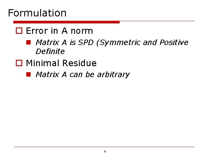
Formulation o Error in A norm n Matrix A is SPD (Symmetric and Positive Definite o Minimal Residue n Matrix A can be arbitrary 4

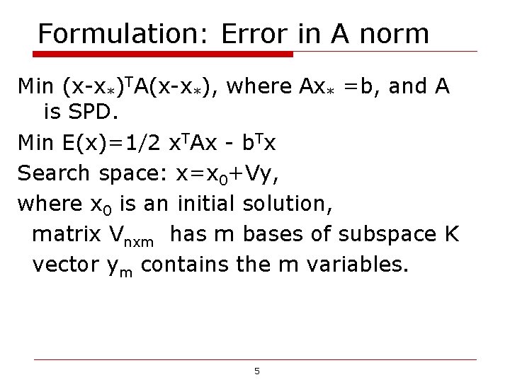
Formulation: Error in A norm Min (x-x*)TA(x-x*), where Ax* =b, and A is SPD. Min E(x)=1/2 x. TAx - b. Tx Search space: x=x 0+Vy, where x 0 is an initial solution, matrix Vnxm has m bases of subspace K vector ym contains the m variables. 5

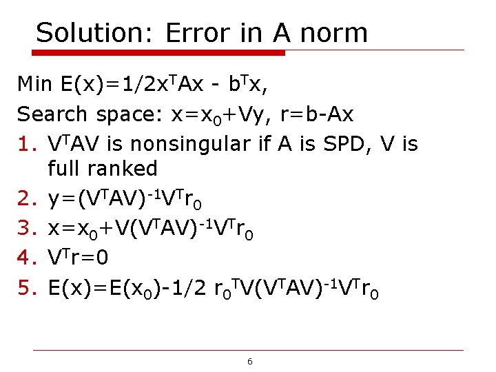
Solution: Error in A norm Min E(x)=1/2 x. TAx - b. Tx, Search space: x=x 0+Vy, r=b-Ax 1. VTAV is nonsingular if A is SPD, V is full ranked 2. y=(VTAV)-1 VTr 0 3. x=x 0+V(VTAV)-1 VTr 0 4. VTr=0 5. E(x)=E(x 0)-1/2 r 0 TV(VTAV)-1 VTr 0 6

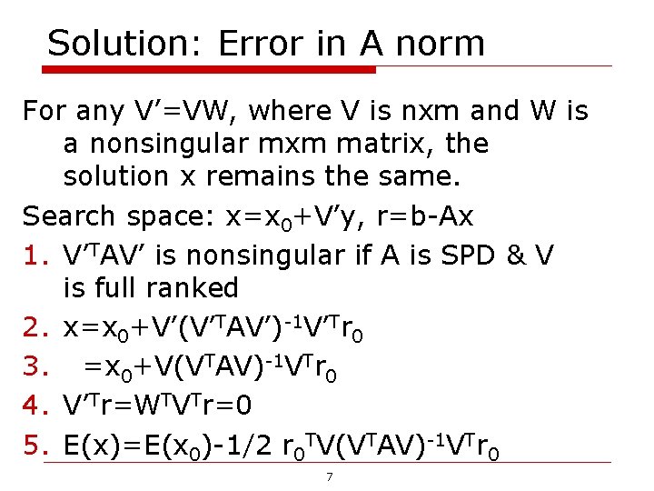
Solution: Error in A norm For any V’=VW, where V is nxm and W is a nonsingular mxm matrix, the solution x remains the same. Search space: x=x 0+V’y, r=b-Ax 1. V’TAV’ is nonsingular if A is SPD & V is full ranked 2. x=x 0+V’(V’TAV’)-1 V’Tr 0 3. =x 0+V(VTAV)-1 VTr 0 4. V’Tr=WTVTr=0 5. E(x)=E(x 0)-1/2 r 0 TV(VTAV)-1 VTr 0 7

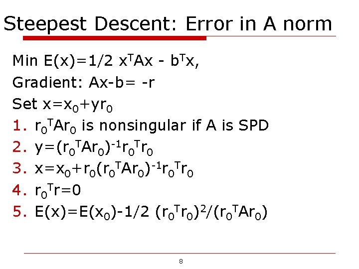
Steepest Descent: Error in A norm Min E(x)=1/2 x. TAx - b. Tx, Gradient: Ax-b= -r Set x=x 0+yr 0 1. r 0 TAr 0 is nonsingular if A is SPD 2. y=(r 0 TAr 0)-1 r 0 Tr 0 3. x=x 0+r 0(r 0 TAr 0)-1 r 0 Tr 0 4. r 0 Tr=0 5. E(x)=E(x 0)-1/2 (r 0 Tr 0)2/(r 0 TAr 0) 8

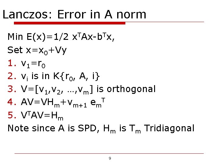
Lanczos: Error in A norm Min E(x)=1/2 x. TAx-b. Tx, Set x=x 0+Vy 1. v 1=r 0 2. vi is in K{r 0, A, i} 3. V=[v 1, v 2, …, vm] is orthogonal 4. AV=VHm+vm+1 em. T 5. VTAV=Hm Note since A is SPD, Hm is Tm Tridiagonal 9

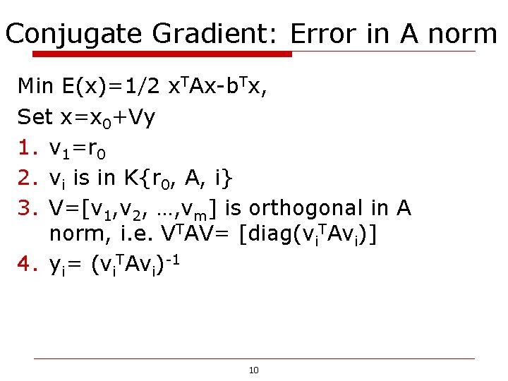
Conjugate Gradient: Error in A norm Min E(x)=1/2 x. TAx-b. Tx, Set x=x 0+Vy 1. v 1=r 0 2. vi is in K{r 0, A, i} 3. V=[v 1, v 2, …, vm] is orthogonal in A norm, i. e. VTAV= [diag(vi. TAvi)] 4. yi= (vi. TAvi)-1 10

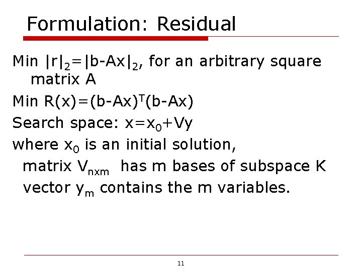
Formulation: Residual Min |r|2=|b-Ax|2, for an arbitrary square matrix A Min R(x)=(b-Ax)T(b-Ax) Search space: x=x 0+Vy where x 0 is an initial solution, matrix Vnxm has m bases of subspace K vector ym contains the m variables. 11

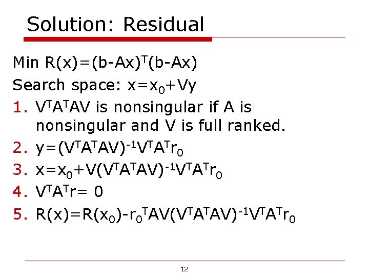
Solution: Residual Min R(x)=(b-Ax)T(b-Ax) Search space: x=x 0+Vy 1. VTATAV is nonsingular if A is nonsingular and V is full ranked. 2. y=(VTATAV)-1 VTATr 0 3. x=x 0+V(VTATAV)-1 VTATr 0 4. VTATr= 0 5. R(x)=R(x 0)-r 0 TAV(VTATAV)-1 VTATr 0 12

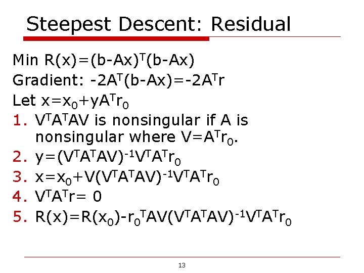
Steepest Descent: Residual Min R(x)=(b-Ax)T(b-Ax) Gradient: -2 AT(b-Ax)=-2 ATr Let x=x 0+y. ATr 0 1. VTATAV is nonsingular if A is nonsingular where V=ATr 0. 2. y=(VTATAV)-1 VTATr 0 3. x=x 0+V(VTATAV)-1 VTATr 0 4. VTATr= 0 5. R(x)=R(x 0)-r 0 TAV(VTATAV)-1 VTATr 0 13

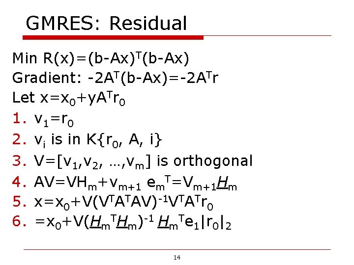
GMRES: Residual Min R(x)=(b-Ax)T(b-Ax) Gradient: -2 AT(b-Ax)=-2 ATr Let x=x 0+y. ATr 0 1. v 1=r 0 2. vi is in K{r 0, A, i} 3. V=[v 1, v 2, …, vm] is orthogonal 4. AV=VHm+vm+1 em. T=Vm+1 Hm 5. x=x 0+V(VTATAV)-1 VTATr 0 6. =x 0+V(Hm. THm)-1 Hm. Te 1|r 0|2 14

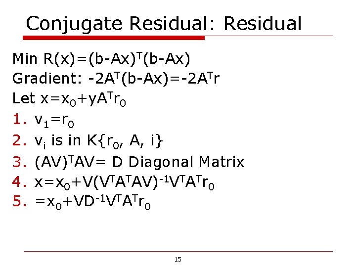
Conjugate Residual: Residual Min R(x)=(b-Ax)T(b-Ax) Gradient: -2 AT(b-Ax)=-2 ATr Let x=x 0+y. ATr 0 1. v 1=r 0 2. vi is in K{r 0, A, i} 3. (AV)TAV= D Diagonal Matrix 4. x=x 0+V(VTATAV)-1 VTATr 0 5. =x 0+VD-1 VTATr 0 15

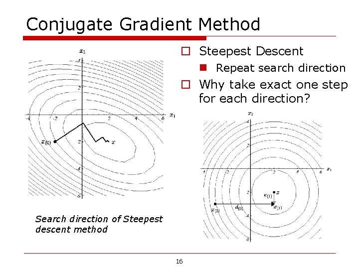
Conjugate Gradient Method o Steepest Descent n Repeat search direction o Why take exact one step for each direction? Search direction of Steepest descent method 16

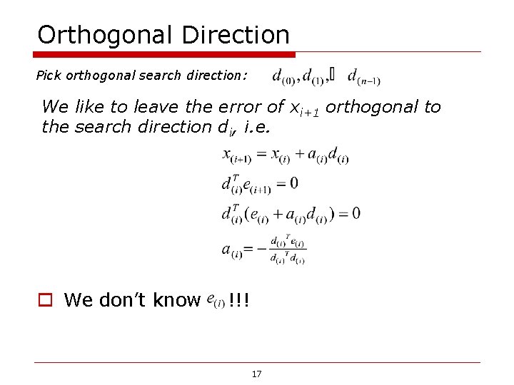
Orthogonal Direction Pick orthogonal search direction: We like to leave the error of xi+1 orthogonal to the search direction di, i. e. o We don’t know !!! 17

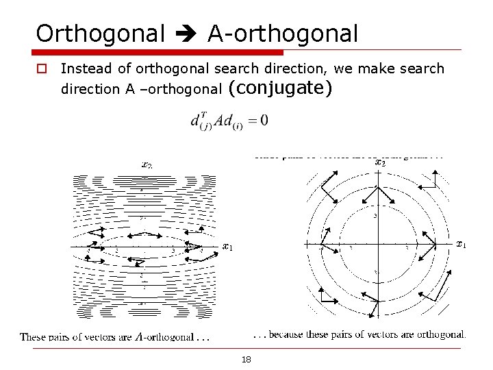
Orthogonal A-orthogonal o Instead of orthogonal search direction, we make search direction A –orthogonal (conjugate) 18

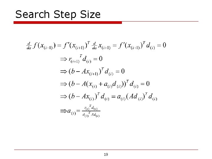
Search Step Size 19

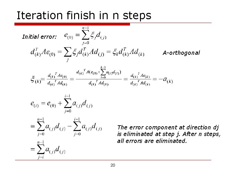
Iteration finish in n steps Initial error: A-orthogonal The error component at direction dj is eliminated at step j. After n steps, all errors are eliminated. 20

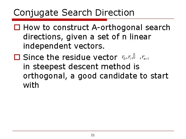
Conjugate Search Direction o How to construct A-orthogonal search directions, given a set of n linear independent vectors. o Since the residue vector in steepest descent method is orthogonal, a good candidate to start with 21

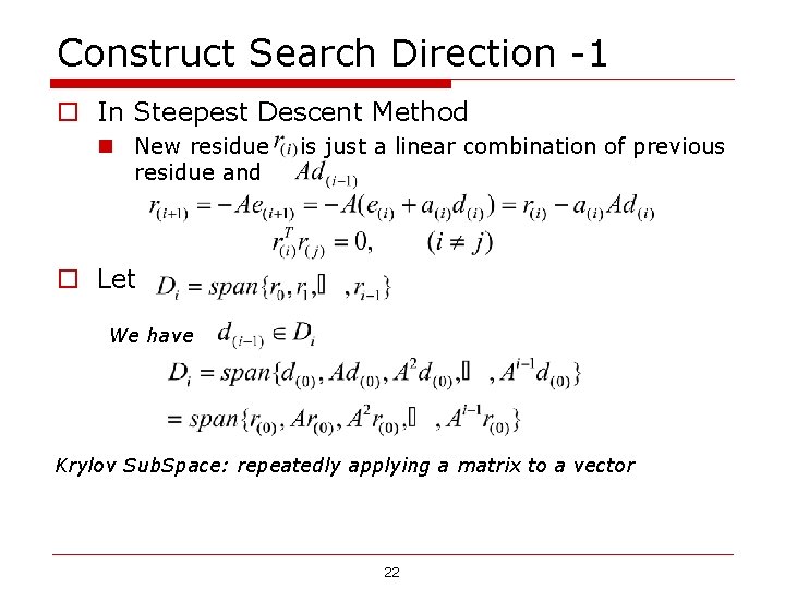
Construct Search Direction -1 o In Steepest Descent Method n New residue and is just a linear combination of previous o Let We have Krylov Sub. Space: repeatedly applying a matrix to a vector 22

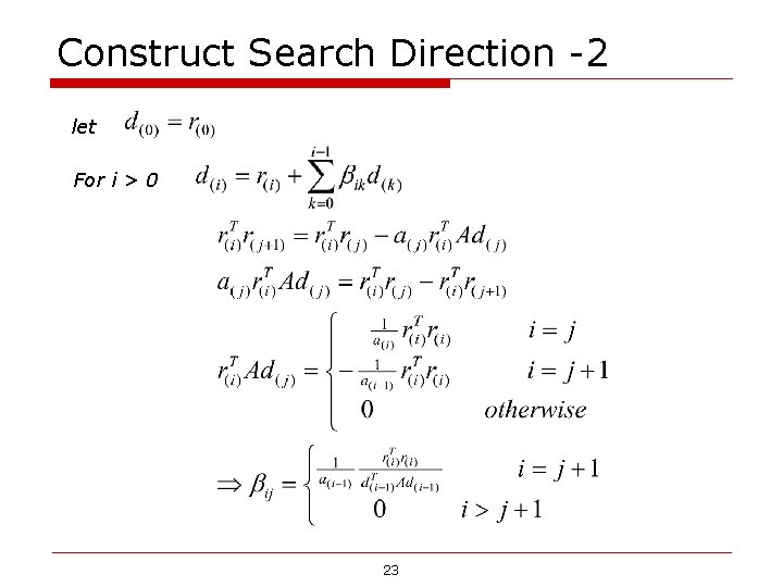
Construct Search Direction -2 let For i > 0 23

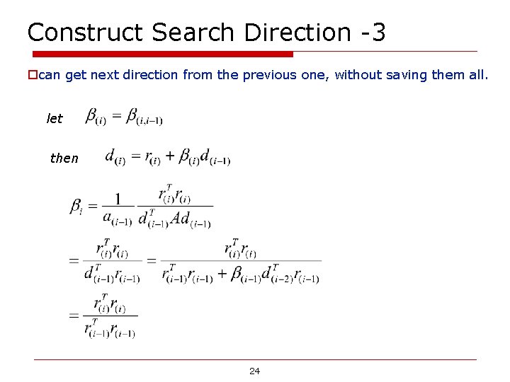
Construct Search Direction -3 ocan get next direction from the previous one, without saving them all. let then 24

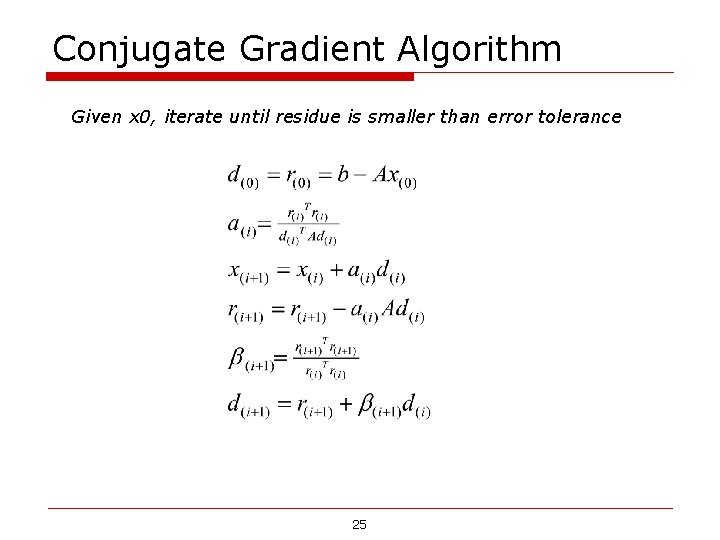
Conjugate Gradient Algorithm Given x 0, iterate until residue is smaller than error tolerance 25

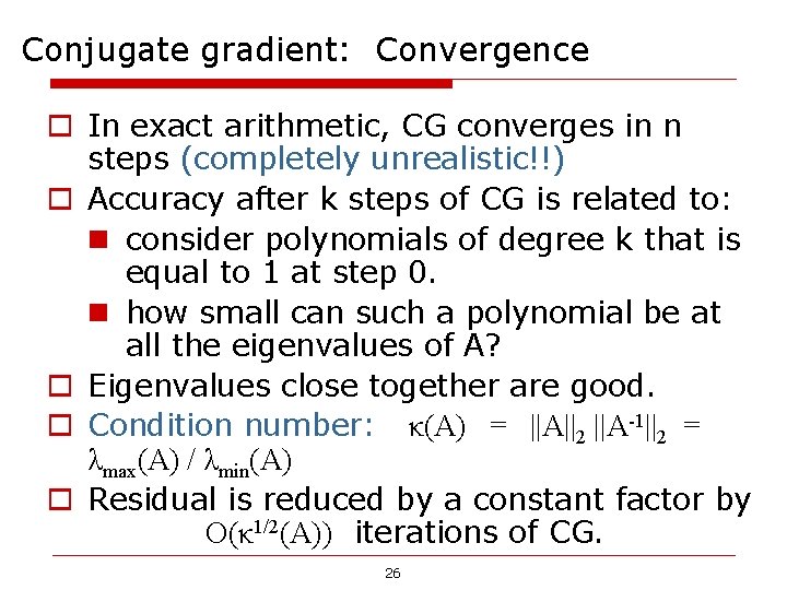
Conjugate gradient: Convergence o In exact arithmetic, CG converges in n steps (completely unrealistic!!) o Accuracy after k steps of CG is related to: n consider polynomials of degree k that is equal to 1 at step 0. n how small can such a polynomial be at all the eigenvalues of A? o Eigenvalues close together are good. o Condition number: κ(A) = ||A||2 ||A-1||2 = λmax(A) / λmin(A) o Residual is reduced by a constant factor by O(κ 1/2(A)) iterations of CG. 26

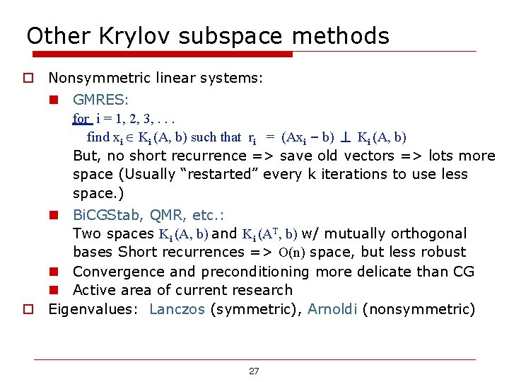
Other Krylov subspace methods o Nonsymmetric linear systems: n GMRES: for i = 1, 2, 3, . . . find xi Ki (A, b) such that ri = (Axi – b) Ki (A, b) But, no short recurrence => save old vectors => lots more space (Usually “restarted” every k iterations to use less space. ) n Bi. CGStab, QMR, etc. : Two spaces Ki (A, b) and Ki (AT, b) w/ mutually orthogonal bases Short recurrences => O(n) space, but less robust n Convergence and preconditioning more delicate than CG n Active area of current research o Eigenvalues: Lanczos (symmetric), Arnoldi (nonsymmetric) 27

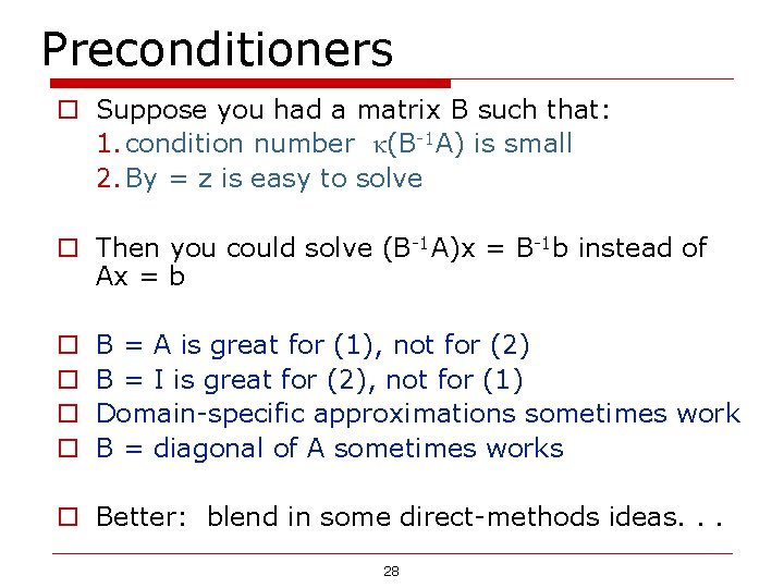
Preconditioners o Suppose you had a matrix B such that: 1. condition number κ(B-1 A) is small 2. By = z is easy to solve o Then you could solve (B-1 A)x = B-1 b instead of Ax = b o o B = A is great for (1), not for (2) B = I is great for (2), not for (1) Domain-specific approximations sometimes work B = diagonal of A sometimes works o Better: blend in some direct-methods ideas. . . 28

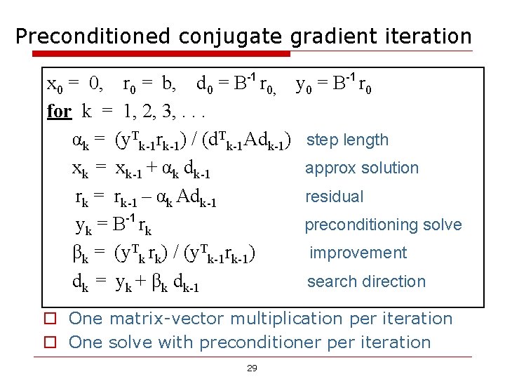
Preconditioned conjugate gradient iteration x 0 = 0, r 0 = b, d 0 = B-1 r 0, y 0 = B-1 r 0 for k = 1, 2, 3, . . . αk = (y. Tk-1 rk-1) / (d. Tk-1 Adk-1) step length xk = xk-1 + αk dk-1 approx solution rk = rk-1 – αk Adk-1 residual yk = B-1 rk preconditioning solve βk = (y. Tk rk) / (y. Tk-1 rk-1) improvement dk = yk + βk dk-1 search direction o One matrix-vector multiplication per iteration o One solve with preconditioner per iteration 29

Outline o Iterative Method n Stationary Iterative Method (SOR, GS, Jacob) n Krylov Method (CG, GMRES) n Multigrid Method 30

What is the multigrid o A multilevel iterative method to solve n Ax=b o Originated in PDEs on geometric grids o Expend the multigrid idea to unstructured problem – Algebraic MG o Geometric multigrid for presenting the basic ideas of the multigrid method. 31

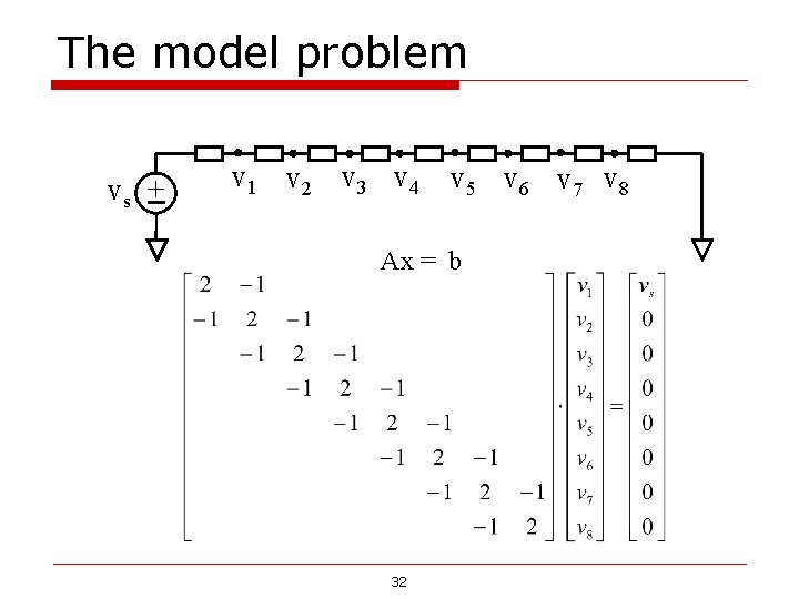
The model problem vs + v 1 v 2 v 3 v 4 v 5 v 6 v 7 v 8 Ax = b 32

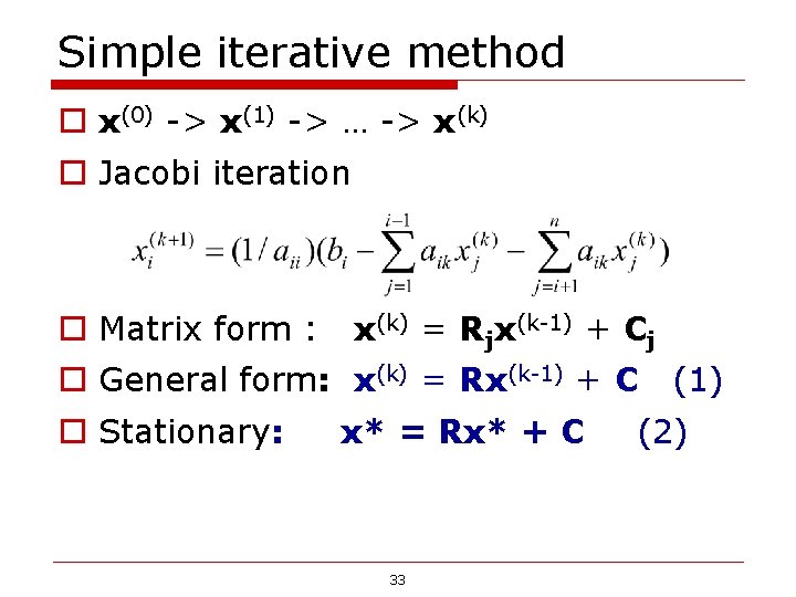
Simple iterative method o x(0) -> x(1) -> … -> x(k) o Jacobi iteration o Matrix form : x(k) = Rjx(k-1) + Cj o General form: x(k) = Rx(k-1) + C o Stationary: x* = Rx* + C 33 (1) (2)

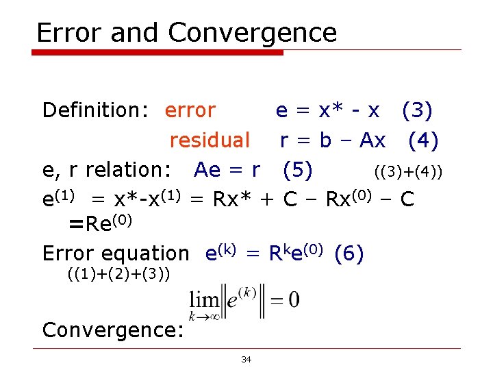
Error and Convergence Definition: error e = x* - x (3) residual r = b – Ax (4) e, r relation: Ae = r (5) ((3)+(4)) e(1) = x*-x(1) = Rx* + C – Rx(0) – C =Re(0) Error equation e(k) = Rke(0) (6) ((1)+(2)+(3)) Convergence: 34

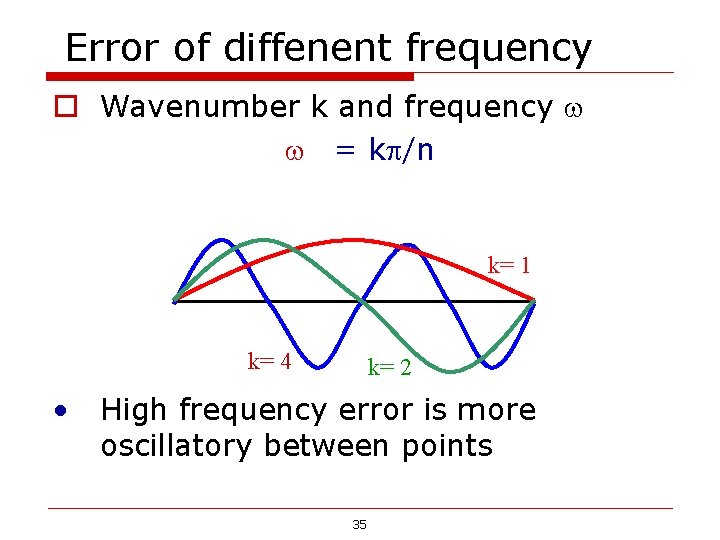
Error of diffenent frequency o Wavenumber k and frequency = k /n k= 1 k= 4 • k= 2 High frequency error is more oscillatory between points 35

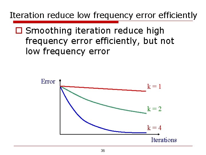
Iteration reduce low frequency error efficiently o Smoothing iteration reduce high frequency error efficiently, but not low frequency error Error k=1 k=2 k=4 Iterations 36

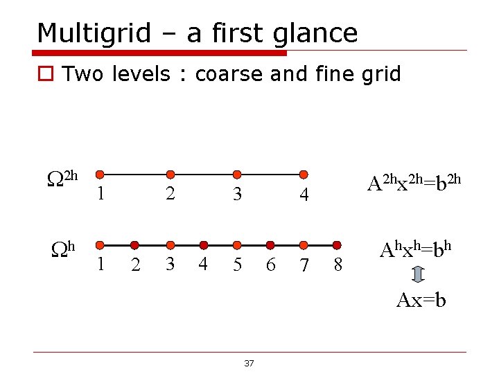
Multigrid – a first glance o Two levels : coarse and fine grid 2 h h 2 1 1 2 3 3 4 A 2 hx 2 h=b 2 h 4 5 6 7 8 Ahxh=bh Ax=b 37

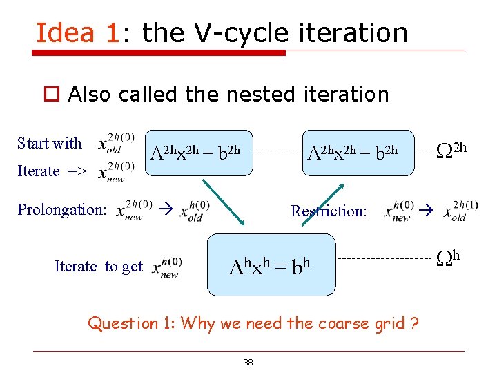
Idea 1: the V-cycle iteration o Also called the nested iteration Start with A 2 hx 2 h = b 2 h Iterate => Prolongation: Iterate to get 2 h A 2 hx 2 h = b 2 h Restriction: Ahxh = bh Question 1: Why we need the coarse grid ? 38 h

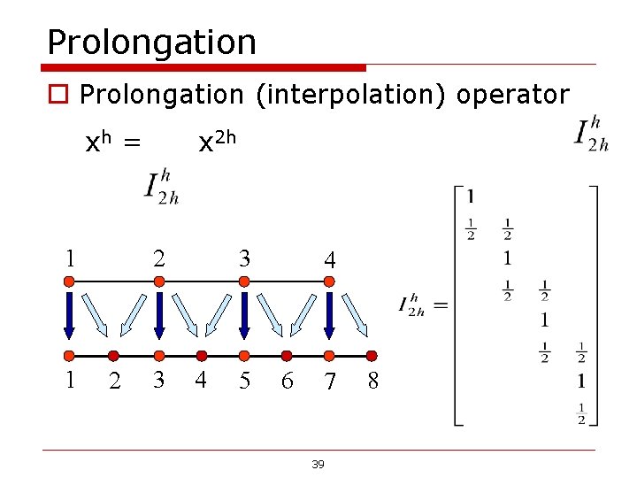
Prolongation o Prolongation (interpolation) operator xh = 2 1 1 x 2 h 2 3 3 4 5 4 6 7 39 8

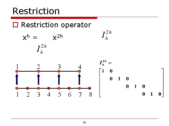
Restriction operator xh = 2 1 1 x 2 h 2 3 3 4 5 4 6 8 7 40

Smoothing o The basic iterations in each level In ph: xphold xphnew o Iteration reduces the error, makes the error smooth geometrically. So the iteration is called smoothing. 41

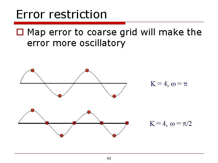
Why multilevel ? o Coarse lever iteration is cheap. o More than this… n Coarse level smoothing reduces the error more efficiently than fine level in some way. n Why ? ( Question 2 ) 42

Error restriction o Map error to coarse grid will make the error more oscillatory K = 4, = /2 43

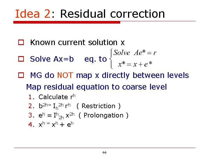
Idea 2: Residual correction o Known current solution x o Solve Ax=b eq. to o MG do NOT map x directly between levels Map residual equation to coarse level 1. 2. 3. 4. Calculate rh b 2 h= Ih 2 h rh ( Restriction ) eh = Ih 2 h x 2 h ( Prolongation ) xh = xh + e h 44

Why residual correction ? o Error is smooth at fine level, but the actual solution may not be. o Prolongation results in a smooth error in fine level, which is suppose to be a good evaluation of the fine level error. o If the solution is not smooth in fine level, prolongation will introduce more high frequency error. 45

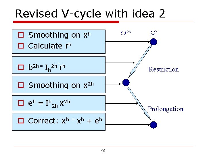
Revised V-cycle with idea 2 o Smoothing on o Calculate rh 2 h xh o b 2 h= Ih 2 h`rh h Restriction o Smoothing on x 2 h o eh = Ih 2 h x 2 h Prolongation o Correct: xh = xh + eh 46

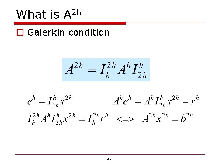
What is A 2 h o Galerkin condition 47

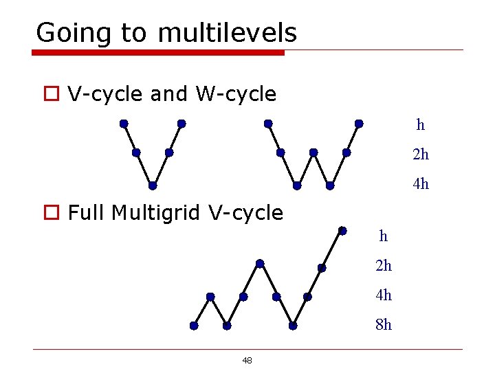
Going to multilevels o V-cycle and W-cycle h 2 h 4 h o Full Multigrid V-cycle h 2 h 4 h 8 h 48

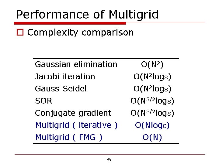
Performance of Multigrid o Complexity comparison Gaussian elimination O(N 2) Jacobi iteration O(N 2 log ) Gauss-Seidel O(N 2 log ) SOR O(N 3/2 log ) Conjugate gradient O(N 3/2 log ) Multigrid ( iterative ) Multigrid ( FMG ) O(Nlog ) O(N) 49

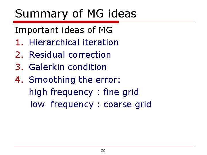
Summary of MG ideas Important ideas of MG 1. Hierarchical iteration 2. Residual correction 3. Galerkin condition 4. Smoothing the error: high frequency : fine grid low frequency : coarse grid 50

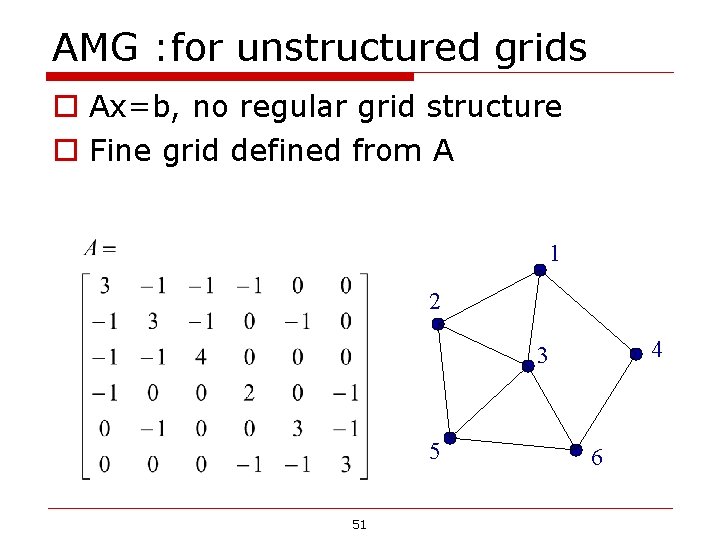
AMG : for unstructured grids o Ax=b, no regular grid structure o Fine grid defined from A 1 2 4 3 5 51 6

Three questions for AMG o How to choose coarse grid o How to define the smoothness of errors o How are interpolation and prolongation done 52

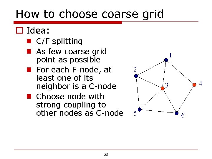
How to choose coarse grid o Idea: n C/F splitting n As few coarse grid point as possible n For each F-node, at least one of its neighbor is a C-node n Choose node with strong coupling to other nodes as C-node 53 1 2 4 3 5 6

How to define the smoothness of error o AMG fundamental concept: Smooth error = small residuals o ||r|| << ||e|| 54

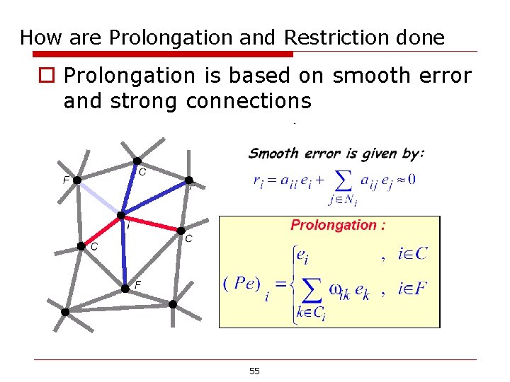
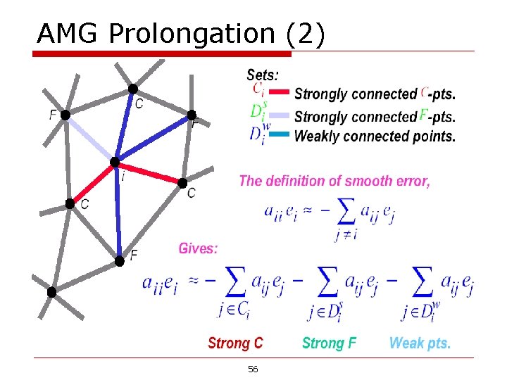
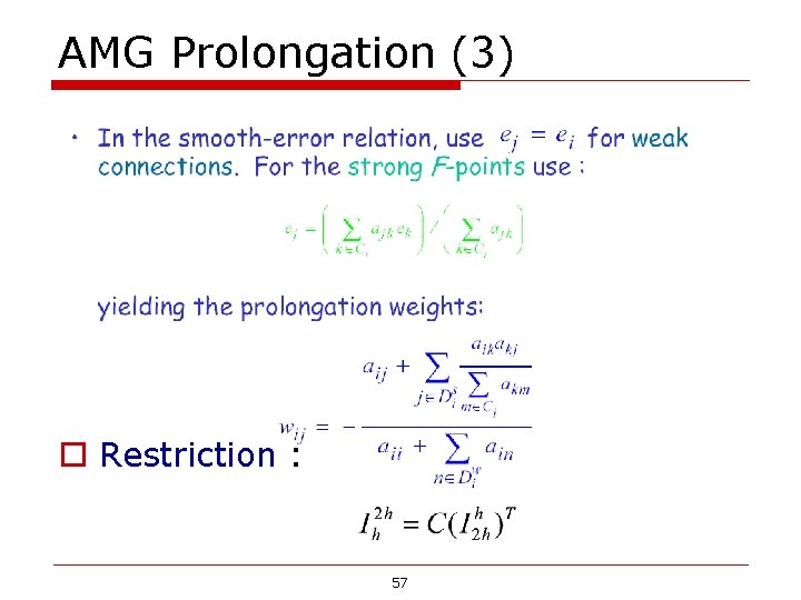
How are Prolongation and Restriction done o Prolongation is based on smooth error and strong connections o Common practice: I 55

AMG Prolongation (2) 56

AMG Prolongation (3) o Restriction : 57

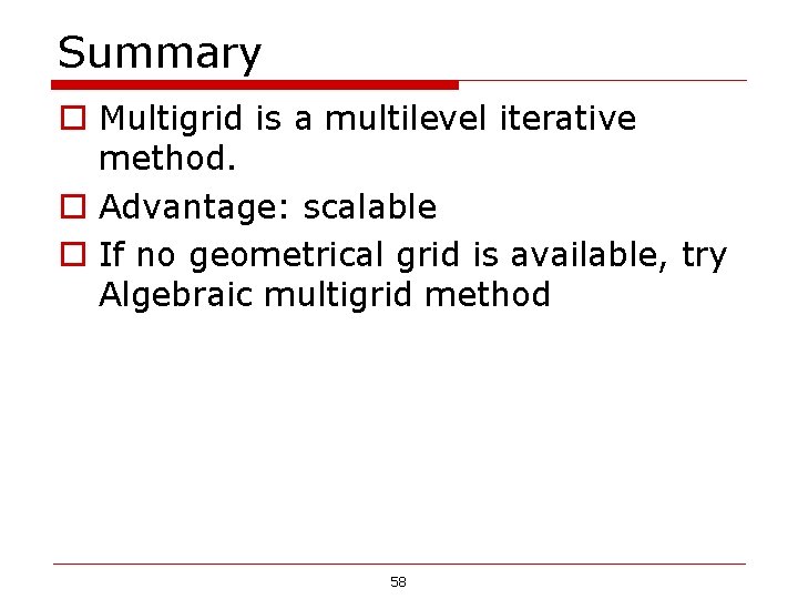
Summary o Multigrid is a multilevel iterative method. o Advantage: scalable o If no geometrical grid is available, try Algebraic multigrid method 58

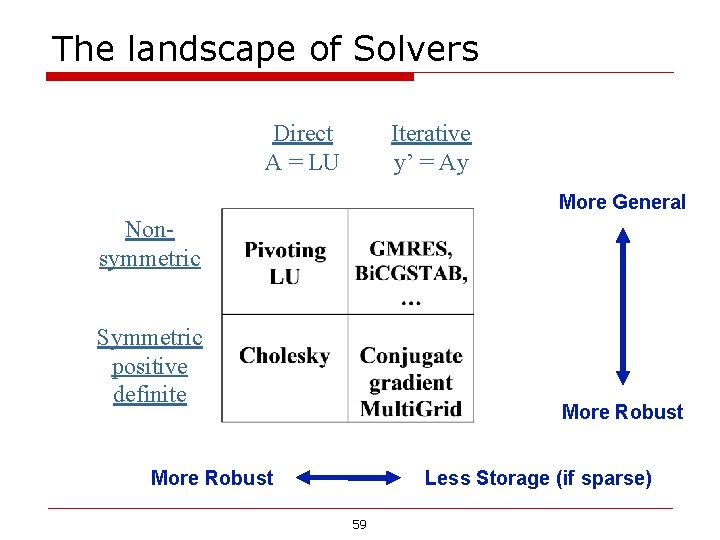
The landscape of Solvers Direct A = LU Iterative y’ = Ay More General Nonsymmetric Symmetric positive definite More Robust Less Storage (if sparse) 59

References o G. H. Golub and C. F. Van Loan, Matrix Computataions, Third Edition, Johns Hopkins, 1996 o Y. Saad, Iterative Methods for Sparse Linear Systems, Second Edition, SIAM, 2003. 60