CSE 182 L 9 Modeling Protein domains using

CSE 182 -L 9 Modeling Protein domains using HMMs

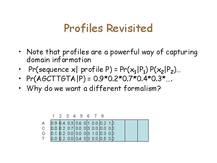
Profiles Revisited • Note that profiles are a powerful way of capturing domain information • Pr(sequence x| profile P) = Pr(x 1|P 1) P(x 2|P 2)… • Pr(AGCTTGTA|P) = 0. 9*0. 2*0. 7*0. 4*0. 3*…. • Why do we want a different formalism? A C G T 1 2 3 4 0. 9 0. 0 0. 1 0. 0 0. 4 0. 2 0. 3 0. 7 0. 0 5 6 7 8 0. 6 0. 0 0. 4 0. 1 0. 3 0. 0 1. 0 0. 2 0. 0 0. 3 0. 5 1. 0 0. 0

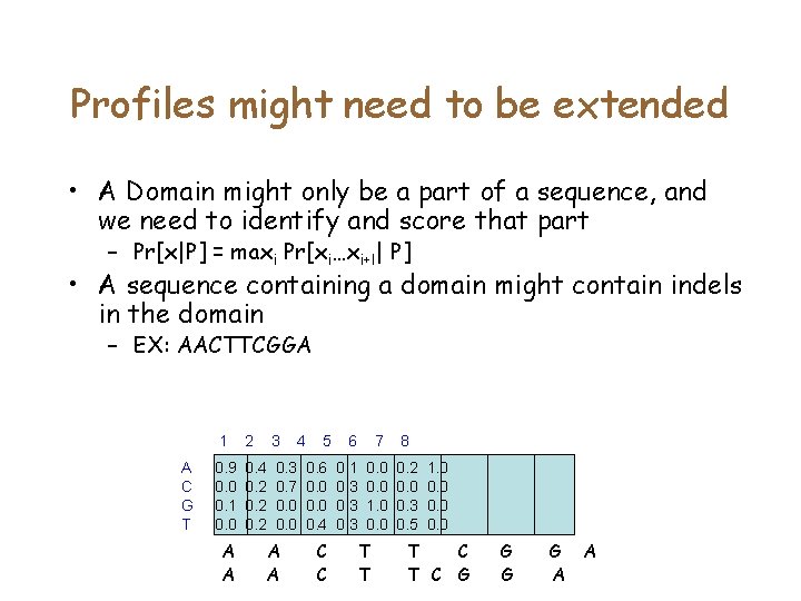
Profiles might need to be extended • A Domain might only be a part of a sequence, and we need to identify and score that part – Pr[x|P] = maxi Pr[xi…xi+l| P] • A sequence containing a domain might contain indels in the domain – EX: AACTTCGGA A C G T 1 2 3 0. 9 0. 0 0. 1 0. 0 0. 4 0. 2 0. 3 0. 7 0. 0 A A 4 5 6 7 8 0. 6 0. 0 0. 4 0. 1 0. 3 0. 0 1. 0 0. 2 0. 0 0. 3 0. 5 C C T T 1. 0 0. 0 T C G G A A

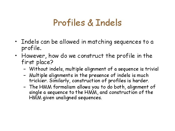
Profiles & Indels • Indels can be allowed in matching sequences to a profile. • However, how do we construct the profile in the first place? – Without indels, multiple alignment of a sequence is trivial – Multiple alignments in the presence of indels is much trickier. Similarly, construction of profiles is harder. – The HMM formalism allows you to do both, alignment of single a sequence to the HMM, and construction of the HMM given unaligned sequences.

Profiles and Compositional signals • • While most protein domains have position dependent properties, other biological signals do not. Ex: 1. Cp. G islands, 2. Signals for protein targeting, transmembrane etc.

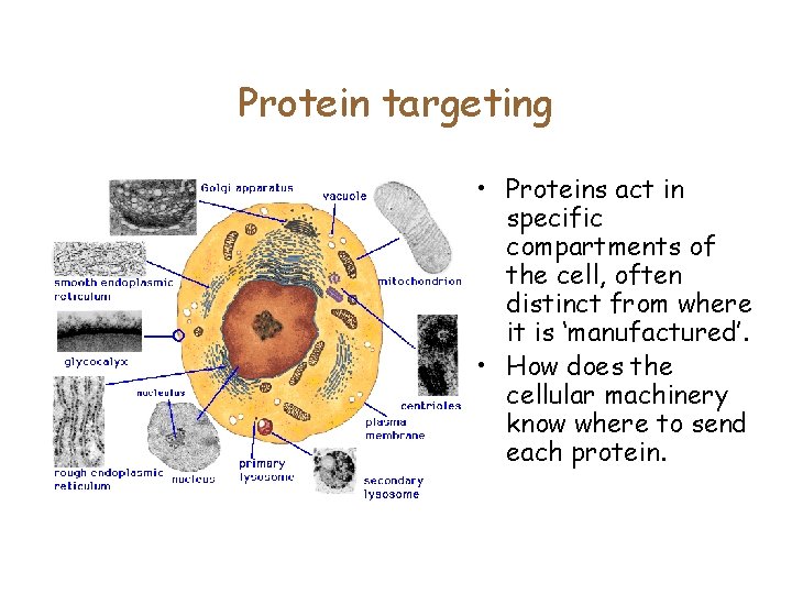
Protein targeting • Proteins act in specific compartments of the cell, often distinct from where it is ‘manufactured’. • How does the cellular machinery know where to send each protein.

Protein targeting • In 1970, Gunter Blobel showed that proteins have an N-terminal signal sequence which directs proteins to the membrane. • Proteins have to be transported to other organelles: nucleus, mitochondria, … • Can we computationally identify the ‘signal’ which distinguishes the cellular compartment?

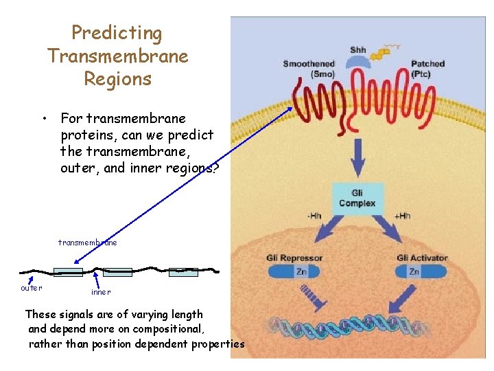
Predicting Transmembrane Regions • For transmembrane proteins, can we predict the transmembrane, outer, and inner regions? transmembrane outer inner These signals are of varying length and depend more on compositional, rather than position dependent properties

The answer is HMMs • Certainly, it is not the only answer! Many other formalisms have been proposed, such as Neural Networks, with varying degree of success.

Revisiting automaton • Recall that Profiles were introduced as a generalization of automata • The OR operator is replaced by a distribution. However, the * operator (Kleene’s closure) has no direct analog. • Instead we introduce probabilities directly into automata.

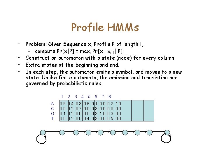
Profile HMMs • • Problem: Given Sequence x, Profile P of length l, – compute Pr[x|P] = maxi Pr[xi…xi+l| P] Construct an automaton with a state (node) for every column Extra states at the beginning and end. In each step, the automaton emits a symbol, and moves to a new state. Unlike finite automata, the emission and transistion are governed by probabilistic rules A C G T 1 2 3 4 0. 9 0. 0 0. 1 0. 0 0. 4 0. 2 0. 3 0. 7 0. 0 5 6 7 8 0. 6 0. 0 0. 4 0. 1 0. 3 0. 0 1. 0 0. 2 0. 0 0. 3 0. 5 1. 0 0. 0

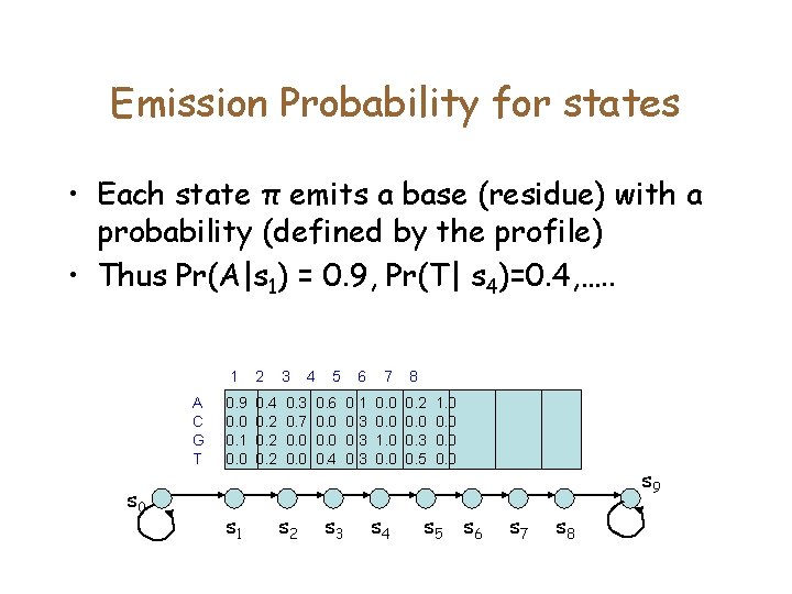
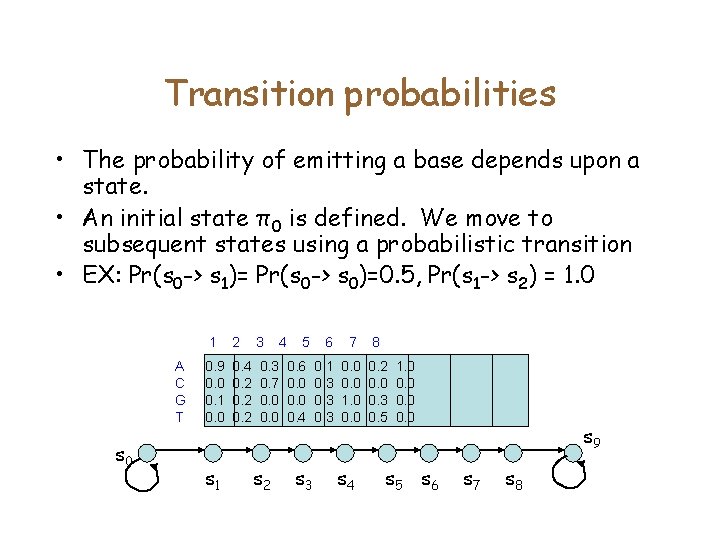
Emission Probability for states • Each state π emits a base (residue) with a probability (defined by the profile) • Thus Pr(A|s 1) = 0. 9, Pr(T| s 4)=0. 4, …. . A C G T s 0 1 2 3 0. 9 0. 0 0. 1 0. 0 0. 4 0. 2 0. 3 0. 7 0. 0 s 1 s 2 4 5 6 7 8 0. 6 0. 0 0. 4 0. 1 0. 3 0. 0 1. 0 0. 2 0. 0 0. 3 0. 5 s 3 s 4 1. 0 0. 0 s 5 s 6 s 9 s 7 s 8

Transition probabilities • The probability of emitting a base depends upon a state. • An initial state π0 is defined. We move to subsequent states using a probabilistic transition • EX: Pr(s 0 -> s 1)= Pr(s 0 -> s 0)=0. 5, Pr(s 1 -> s 2) = 1. 0 A C G T s 0 1 2 3 0. 9 0. 0 0. 1 0. 0 0. 4 0. 2 0. 3 0. 7 0. 0 s 1 s 2 4 5 6 7 8 0. 6 0. 0 0. 4 0. 1 0. 3 0. 0 1. 0 0. 2 0. 0 0. 3 0. 5 s 3 s 4 1. 0 0. 0 s 5 s 6 s 9 s 7 s 8

Emission of a sequence • What is the probability that the automaton emitted the sequence x 1. . xn • The problem becomes easier if we know the sequence of states π=π0. . πn that the automaton was in

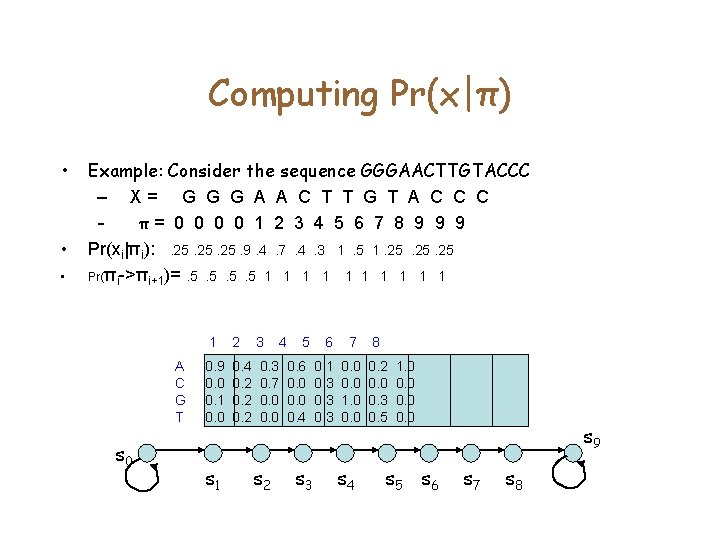
Computing Pr(x|π) • • • Example: Consider the sequence GGGAACTTGTACCC – X= G G G A A C T T G T A C C C – π= 0 0 1 2 3 4 5 6 7 8 9 9 9 Pr(xi|πi): . 25. 25. 9. 4. 7. 4. 3 1. 5 1. 25. 25 Pr(πi->πi+1)=. 5. 5 1 1 1 1 1 A C G T s 0 1 2 3 0. 9 0. 0 0. 1 0. 0 0. 4 0. 2 0. 3 0. 7 0. 0 s 1 s 2 4 5 6 7 8 0. 6 0. 0 0. 4 0. 1 0. 3 0. 0 1. 0 0. 2 0. 0 0. 3 0. 5 s 3 s 4 1. 0 0. 0 s 5 s 6 s 9 s 7 s 8

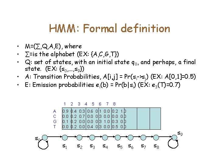
HMM: Formal definition • M=(∑, Q, A, E), where • ∑=is the alphabet (EX: {A, C, G, T}) • Q: set of states, with an initial state q 0, and perhaps, a final state. (EX: {s 0, …, s 9}) • A: Transition Probabilities, A[i, j] = Pr(si->sj) (EX: A[0, 1]=0. 5) • E: Emission probabilities ei(b) = Pr(b|si) (EX: e 3(T)=0. 7) A C G T s 0 1 2 3 0. 9 0. 0 0. 1 0. 0 0. 4 0. 2 0. 3 0. 7 0. 0 s 1 s 2 4 5 6 7 8 0. 6 0. 0 0. 4 0. 1 0. 3 0. 0 1. 0 0. 2 0. 0 0. 3 0. 5 s 3 s 4 1. 0 0. 0 s 5 s 6 s 9 s 7 s 8

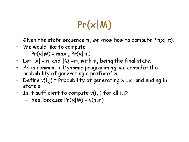
Pr(x|M) • Given the state sequence π, we know how to compute Pr(x| π). • We would like to compute – Pr(x|M) = max π Pr(x| π) • Let |x| = n, and |Q|=m, with sm being the final state. • As is common in Dynamic programming, we consider the probability of generating a prefix of x • Define v(i, j) = Probability of generating x 1. . xi, and ending in state sj • Is it sufficient to compute v(i, j) for all i, j? – Yes, because Pr(x|M) = v(n, m)

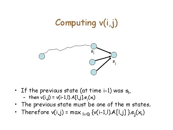
Computing v(i, j) sl sj • If the previous state (at time i-1) was sl, – then v(i, j) = v(i-1, l). A[l, j]. ej(xi) • The previous state must be one of the m states. • Therefore v(i, j) = max l Q {v(i-1, l). A[l, j] }. ej(xi)

The Viterbi Algorithm • v(i, j) = max l Q {v(i-1, l). A[l, j] }. ej(xi) • We take logarithms and an approximation to maintain precision – S(i, j) = log(ej(xi)) + max l Q{ S[i-1, l] + log(A[l, j] ) } • The Viterbi Algorithm • For i = 1. . n – For j = 1. . M – S(i, j) = log(ej(xi)) + max l Q{ S[i-1, l] + log(A[l, j] ) }

Probability of being in specific states • What is the probability that we were in state k at step I? Pr[All paths that passed through state k at step I, and emitted x] Pr[All paths that emitted x]