CS 440ECE 448 Lecture 24 Hidden Markov Models

CS 440/ECE 448 Lecture 24: Hidden Markov Models Slides by Svetlana Lazebnik, 11/2016 Modified by Mark Hasegawa-Johnson, 11/2017

Probabilistic reasoning over time • So far, we’ve mostly dealt with episodic environments • Exceptions: games with multiple moves, planning • In particular, the Bayesian networks we’ve seen so far describe static situations • Each random variable gets a single fixed value in a single problem instance • Now we consider the problem of describing probabilistic environments that evolve over time • Examples: robot localization, human activity detection, tracking, speech recognition, machine translation,

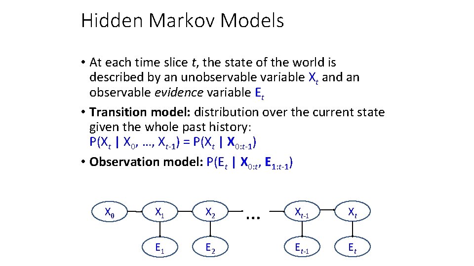
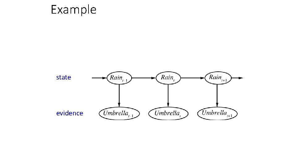
Hidden Markov Models • At each time slice t, the state of the world is described by an unobservable variable Xt and an observable evidence variable Et • Transition model: distribution over the current state given the whole past history: P(Xt | X 0, …, Xt-1) = P(Xt | X 0: t-1) • Observation model: P(Et | X 0: t, E 1: t-1) X 0 X 1 X 2 E 1 E 2 … Xt-1 Xt Et-1 Et

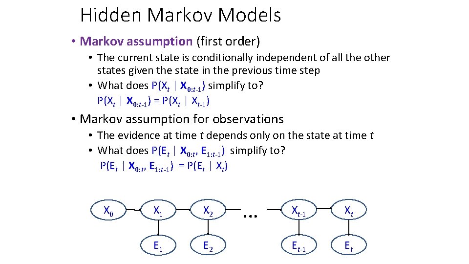
Hidden Markov Models • Markov assumption (first order) • The current state is conditionally independent of all the other states given the state in the previous time step • What does P(Xt | X 0: t-1) simplify to? P(Xt | X 0: t-1) = P(Xt | Xt-1) • Markov assumption for observations • The evidence at time t depends only on the state at time t • What does P(Et | X 0: t, E 1: t-1) simplify to? P(Et | X 0: t, E 1: t-1) = P(Et | Xt) X 0 X 1 X 2 E 1 E 2 … Xt-1 Xt Et-1 Et

Example state evidence

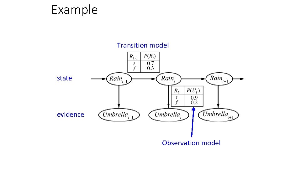
Example Transition model state evidence Observation model

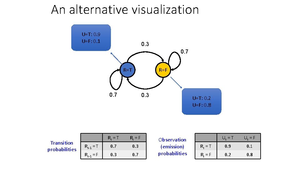
An alternative visualization U=T: 0. 9 U=F: 0. 1 0. 3 0. 7 R=T R=F 0. 7 Transition probabilities 0. 3 Rt = T Rt = F Rt-1 = T 0. 7 0. 3 Rt-1 = F 0. 3 0. 7 U=T: 0. 2 U=F: 0. 8 Observation (emission) probabilities Ut = T Ut = F Rt = T 0. 9 0. 1 Rt = F 0. 2 0. 8

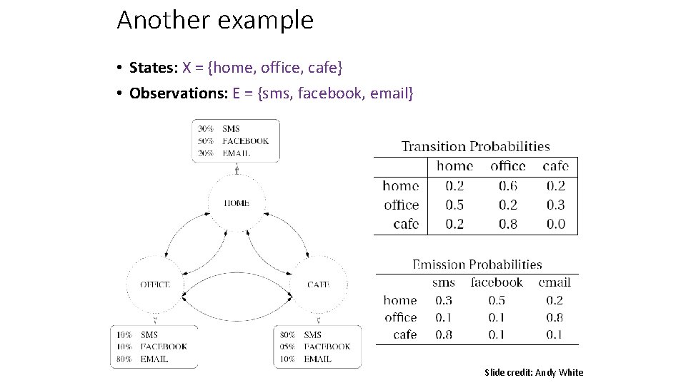
Another example • States: X = {home, office, cafe} • Observations: E = {sms, facebook, email} Slide credit: Andy White

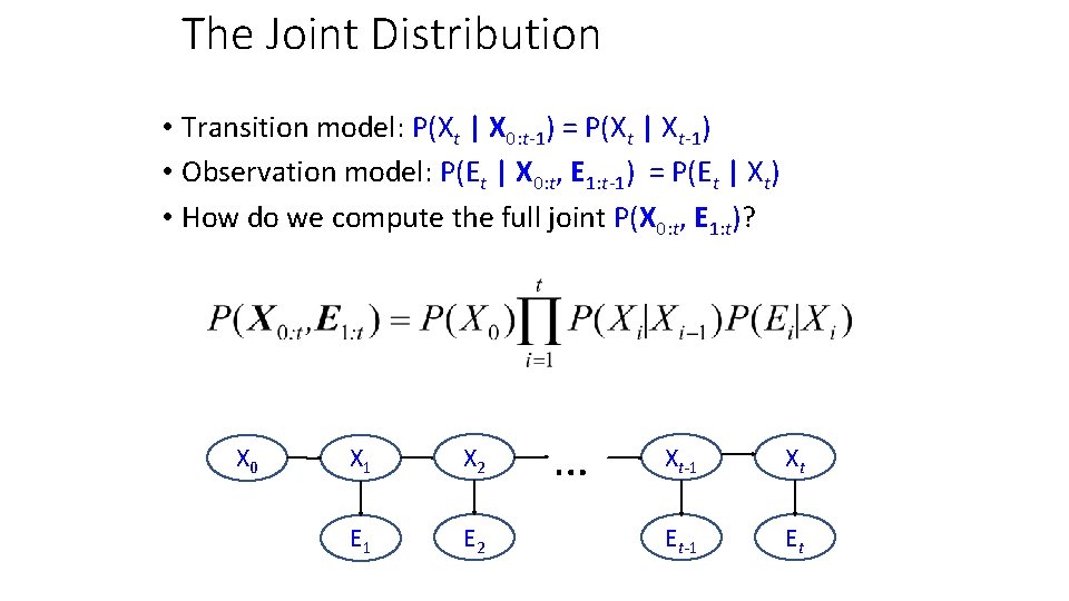
The Joint Distribution • Transition model: P(Xt | X 0: t-1) = P(Xt | Xt-1) • Observation model: P(Et | X 0: t, E 1: t-1) = P(Et | Xt) • How do we compute the full joint P(X 0: t, E 1: t)? X 0 X 1 X 2 E 1 E 2 … Xt-1 Xt Et-1 Et

Review: Bayes net inference • Computational complexity • Special cases • Parameter learning

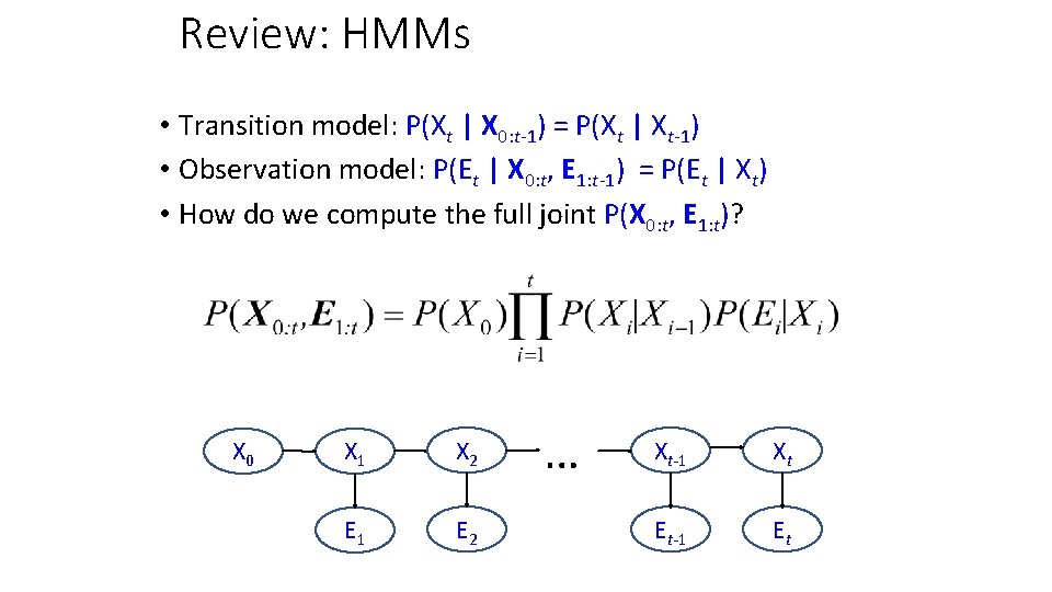
Review: HMMs • Transition model: P(Xt | X 0: t-1) = P(Xt | Xt-1) • Observation model: P(Et | X 0: t, E 1: t-1) = P(Et | Xt) • How do we compute the full joint P(X 0: t, E 1: t)? X 0 X 1 X 2 E 1 E 2 … Xt-1 Xt Et-1 Et

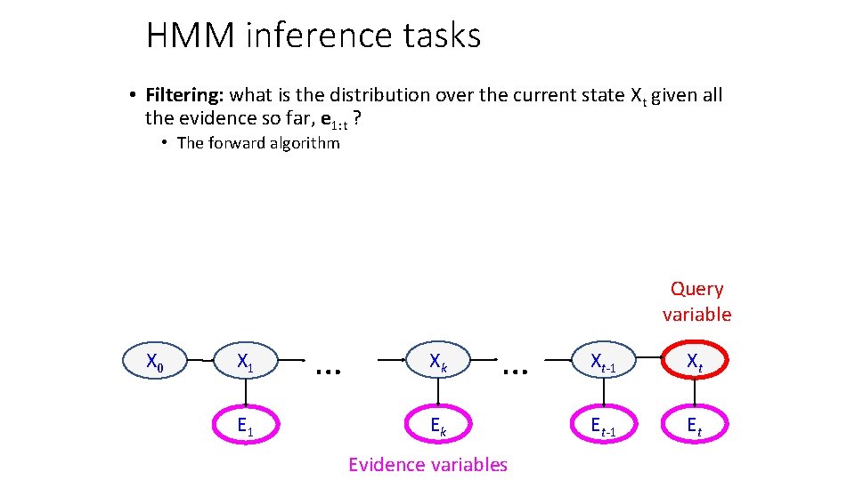
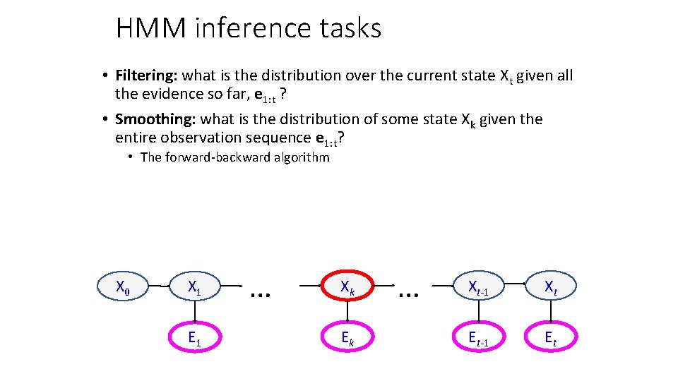
HMM inference tasks • Filtering: what is the distribution over the current state Xt given all the evidence so far, e 1: t ? • The forward algorithm Query variable X 0 X 1 E 1 … Xk … Ek Evidence variables Xt-1 Xt Et-1 Et

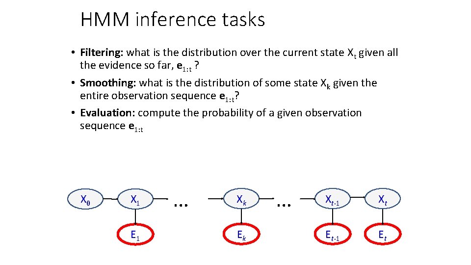
HMM inference tasks • Filtering: what is the distribution over the current state Xt given all the evidence so far, e 1: t ? • Smoothing: what is the distribution of some state Xk given the entire observation sequence e 1: t? • The forward-backward algorithm X 0 X 1 E 1 … Xk Ek … Xt-1 Xt Et-1 Et

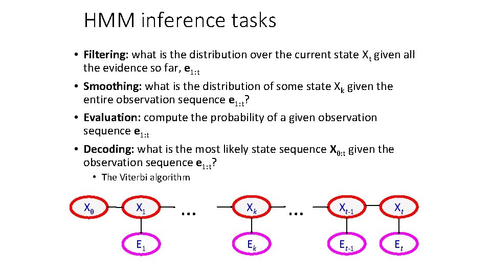
HMM inference tasks • Filtering: what is the distribution over the current state Xt given all the evidence so far, e 1: t ? • Smoothing: what is the distribution of some state Xk given the entire observation sequence e 1: t? • Evaluation: compute the probability of a given observation sequence e 1: t X 0 X 1 E 1 … Xk Ek … Xt-1 Xt Et-1 Et

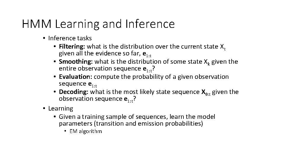
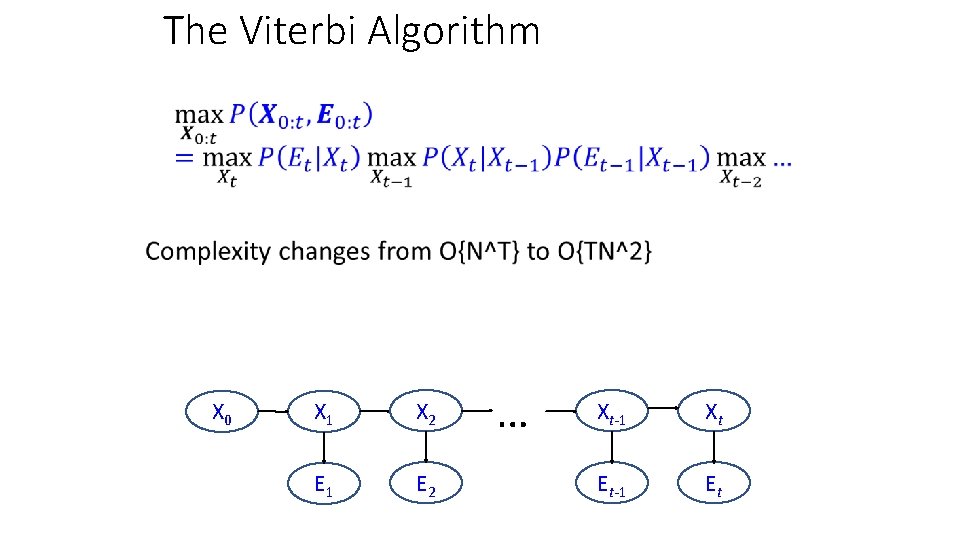
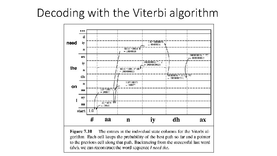
HMM inference tasks • Filtering: what is the distribution over the current state Xt given all the evidence so far, e 1: t • Smoothing: what is the distribution of some state Xk given the entire observation sequence e 1: t? • Evaluation: compute the probability of a given observation sequence e 1: t • Decoding: what is the most likely state sequence X 0: t given the observation sequence e 1: t? • The Viterbi algorithm X 0 X 1 E 1 … Xk Ek … Xt-1 Xt Et-1 Et

HMM Learning and Inference • Inference tasks • Filtering: what is the distribution over the current state Xt given all the evidence so far, e 1: t • Smoothing: what is the distribution of some state Xk given the entire observation sequence e 1: t? • Evaluation: compute the probability of a given observation sequence e 1: t • Decoding: what is the most likely state sequence X 0: t given the observation sequence e 1: t? • Learning • Given a training sample of sequences, learn the model parameters (transition and emission probabilities) • EM algorithm

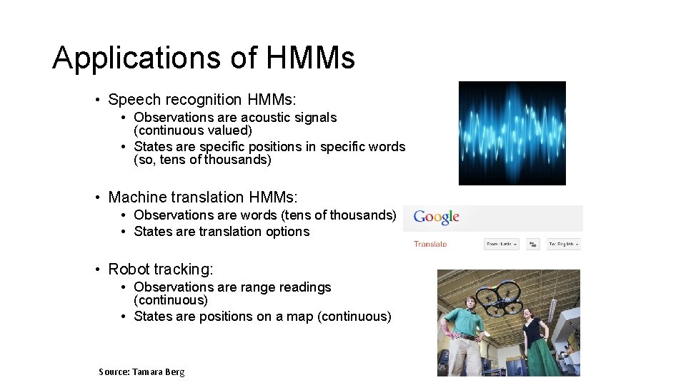
Applications of HMMs • Speech recognition HMMs: • Observations are acoustic signals (continuous valued) • States are specific positions in specific words (so, tens of thousands) • Machine translation HMMs: • Observations are words (tens of thousands) • States are translation options • Robot tracking: • Observations are range readings (continuous) • States are positions on a map (continuous) Source: Tamara Berg

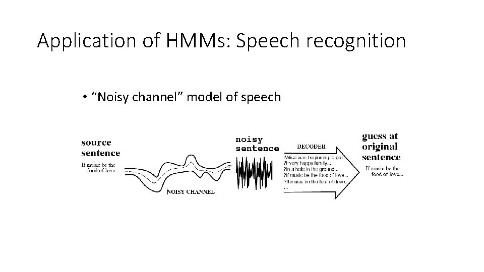
Application of HMMs: Speech recognition • “Noisy channel” model of speech

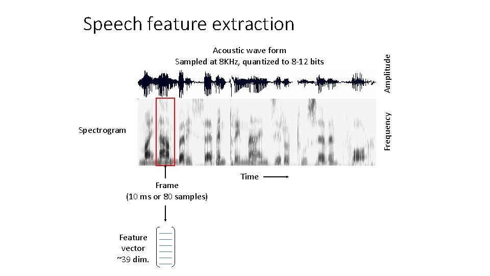
Frequency Acoustic wave form Sampled at 8 KHz, quantized to 8 -12 bits Spectrogram Frame (10 ms or 80 samples) Feature vector ~39 dim. Amplitude Speech feature extraction Time

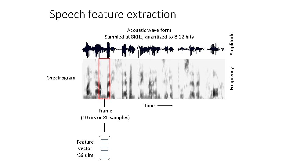
Frequency Acoustic wave form Sampled at 8 KHz, quantized to 8 -12 bits Amplitude Speech feature extraction Spectrogram Frame (10 ms or 80 samples) Feature vector ~39 dim. Time

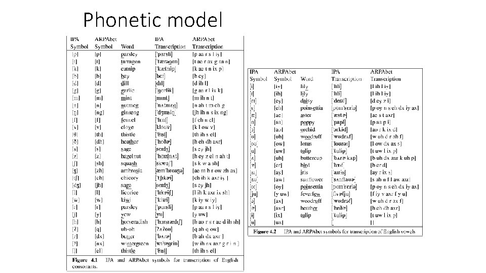
Phonetic model • Phones: speech sounds • Phonemes: groups of speech sounds that have a unique meaning/function in a language (e. g. , there are several different ways to pronounce “t”)

Phonetic model

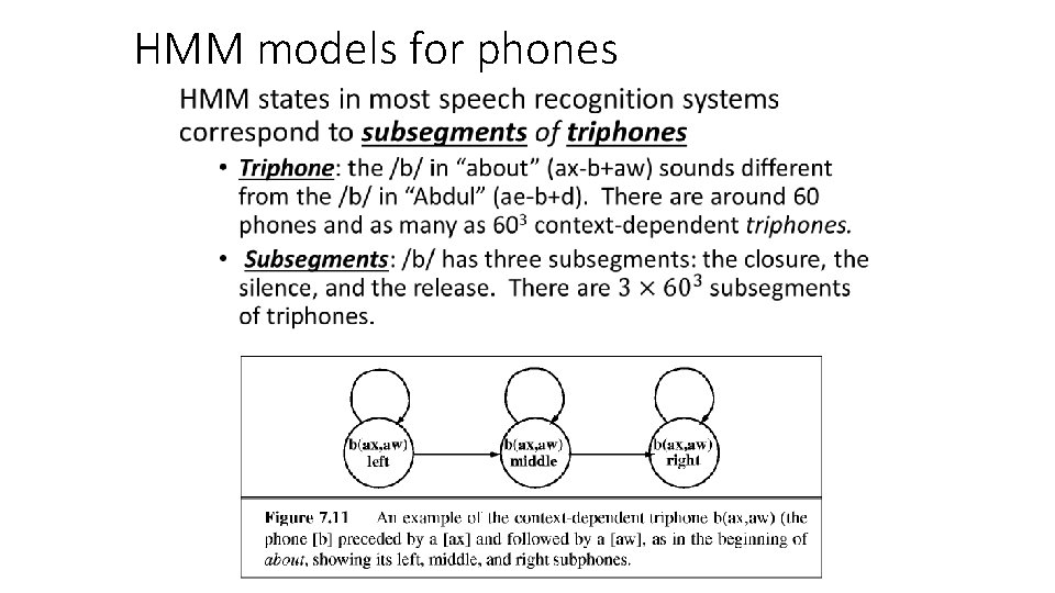
HMM models for phones •

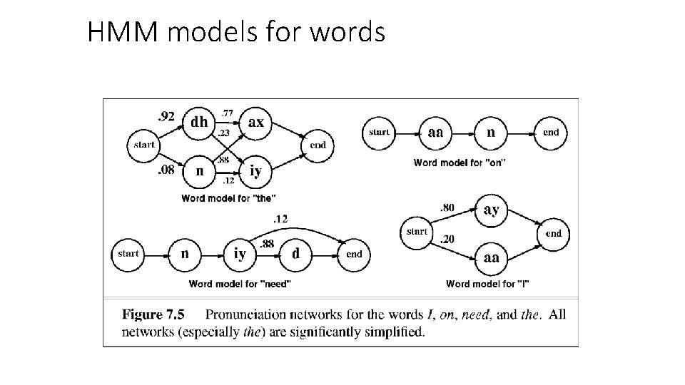
HMM models for words

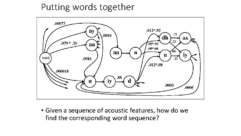
Putting words together • Given a sequence of acoustic features, how do we find the corresponding word sequence?

The Viterbi Algorithm • X 0 X 1 X 2 E 1 E 2 … Xt-1 Xt Et-1 Et

Decoding with the Viterbi algorithm

For more information • CS 447: Natural Language Processing • ECE 417: Multimedia Signal Processing • ECE 594: Mathematical Models of Language • Linguistics 506: Computational Linguistics • D. Jurafsky and J. Martin, “Speech and Language Processing, ” 2 nd ed. , Prentice Hall, 2008