COST MANAGEMENT Don R Hansen Maryanne M Mowen

COST MANAGEMENT Don R. Hansen Maryanne M. Mowen PPT 3 -1

Chapter Three Activity Cost Behavior PPT 3 -2

Learning Objectives l Define and describe fixed, variable, and mixed costs. l Explain the use of resources and activities and their relationship to cost behavior. l Separate mixed costs into their fixed and variable components using the high-low method, the scatterplot method, and the method of least squares. PPT 3 -3

Learning Objectives (continued) l Evaluate the reliability of the cost formula. l Explain how multiple regression can be used to assess cost behavior l Discuss the use of managerial judgment in determining cost behavior. PPT 3 -4

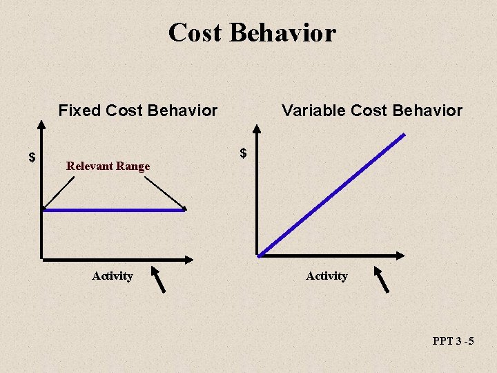
Cost Behavior Fixed Cost Behavior $ Relevant Range Activity Variable Cost Behavior $ Activity PPT 3 -5

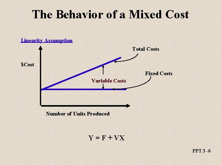
The Behavior of a Mixed Cost Linearity Assumption Total Costs $Cost Fixed Costs Variable Costs Number of Units Produced Y = F + VX PPT 3 -6

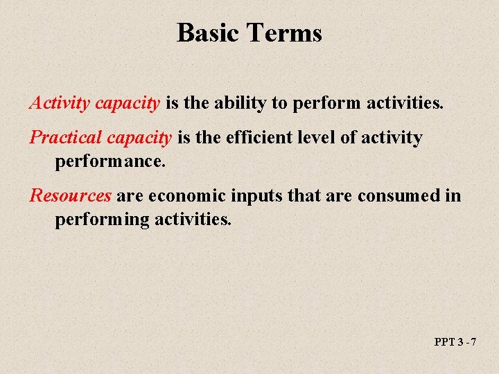
Basic Terms Activity capacity is the ability to perform activities. Practical capacity is the efficient level of activity performance. Resources are economic inputs that are consumed in performing activities. PPT 3 -7

Types of Fixed Resources l Flexible Resources l Committed Resources l Discretionary Fixed Costs PPT 3 -8

Flexible Resources Flexible resources are supplied as used and needed. They are acquired from outside sources, where the terms of acquisition do not require any long-term commitment for any given amount of the resource. Example: Materials and energy PPT 3 -9

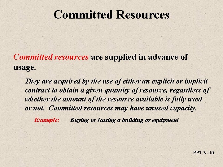
Committed Resources Committed resources are supplied in advance of usage. They are acquired by the use of either an explicit or implicit contract to obtain a given quantity of resource, regardless of whether the amount of the resource available is fully used or not. Committed resources may have unused capacity. Example: Buying or leasing a building or equipment PPT 3 -10

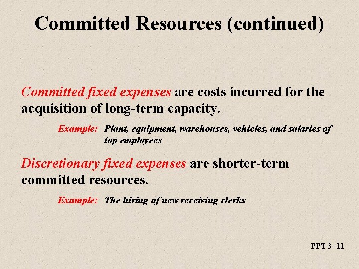
Committed Resources (continued) Committed fixed expenses are costs incurred for the acquisition of long-term capacity. Example: Plant, equipment, warehouses, vehicles, and salaries of top employees Discretionary fixed expenses are shorter-term committed resources. Example: The hiring of new receiving clerks PPT 3 -11

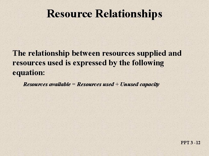
Resource Relationships The relationship between resources supplied and resources used is expressed by the following equation: Resources available = Resources used + Unused capacity PPT 3 -12

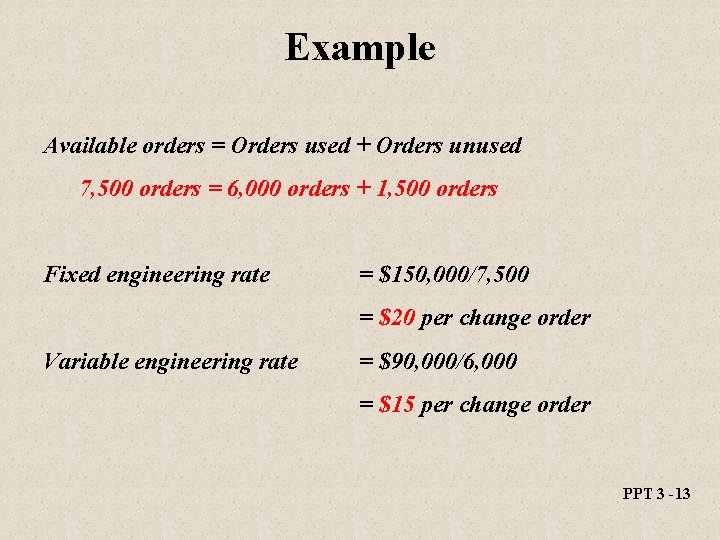
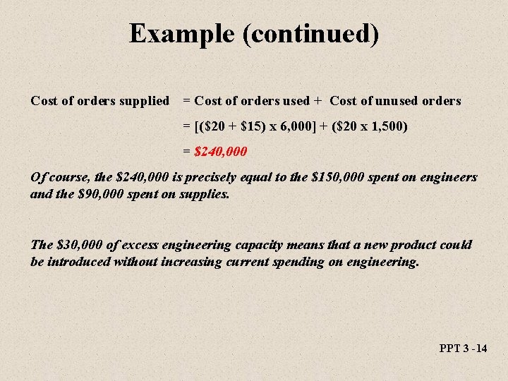
Example Available orders = Orders used + Orders unused 7, 500 orders = 6, 000 orders + 1, 500 orders Fixed engineering rate = $150, 000/7, 500 = $20 per change order Variable engineering rate = $90, 000/6, 000 = $15 per change order PPT 3 -13

Example (continued) Cost of orders supplied = Cost of orders used + Cost of unused orders = [($20 + $15) x 6, 000] + ($20 x 1, 500) = $240, 000 Of course, the $240, 000 is precisely equal to the $150, 000 spent on engineers and the $90, 000 spent on supplies. The $30, 000 of excess engineering capacity means that a new product could be introduced without increasing current spending on engineering. PPT 3 -14

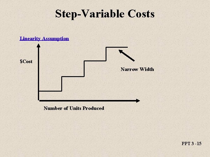
Step-Variable Costs Linearity Assumption $Cost Narrow Width Number of Units Produced PPT 3 -15

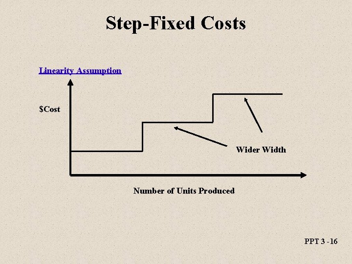
Step-Fixed Costs Linearity Assumption $Cost Wider Width Number of Units Produced PPT 3 -16

Methods for Measuring the Fixed and Variable Components of a Mixed Cost l The High-Low Method l Scatterplot Method l The Method of Least Squares PPT 3 -17

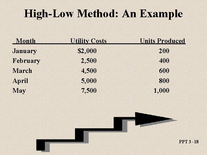
High-Low Method: An Example Month January February March April May Utility Costs $2, 000 2, 500 4, 500 5, 000 7, 500 Units Produced 200 400 600 800 1, 000 PPT 3 -18

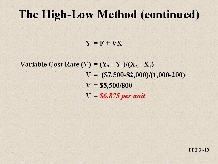
The High-Low Method (continued) Y = F + VX Variable Cost Rate (V) V V V = (Y 2 - Y 1)/(X 2 - X 1) = ($7, 500 -$2, 000)/(1, 000 -200) = $5, 500/800 = $6. 875 per unit PPT 3 -19

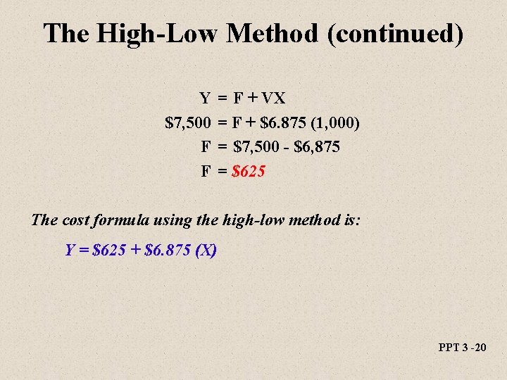
The High-Low Method (continued) Y $7, 500 F F = F + VX = F + $6. 875 (1, 000) = $7, 500 - $6, 875 = $625 The cost formula using the high-low method is: Y = $625 + $6. 875 (X) PPT 3 -20

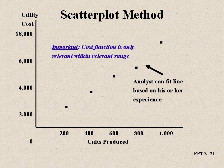
Utility Cost Scatterplot Method . $8, 000 6, 000 Important: Cost function is only relevant within relevant range 4, 000 2, 000 . 200 0 . . . Analyst can fit line based on his or her experience 400 600 800 Units Produced 1, 000 PPT 3 -21

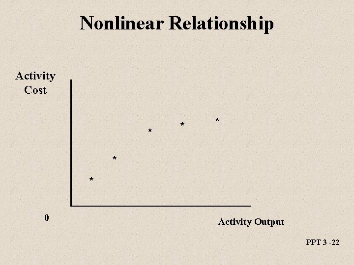
Nonlinear Relationship Activity Cost * * * 0 Activity Output PPT 3 -22

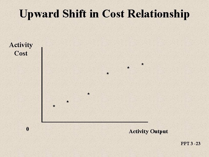
Upward Shift in Cost Relationship Activity Cost * * * 0 * Activity Output PPT 3 -23

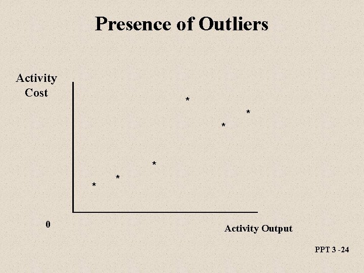
Presence of Outliers Activity Cost * * * 0 * Activity Output PPT 3 -24

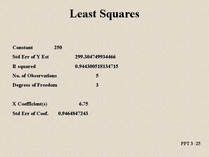
Least Squares Constant 250 Std Err of Y Est 299. 304749934466 R squared 0. 944300518134715 No. of Observations 5 Degrees of Freedom 3 X Coefficient(s) 6. 75 Std Err of Coef. 0. 9464847243 PPT 3 -25

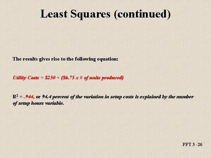
Least Squares (continued) The results gives rise to the following equation: Utility Costs = $250 + ($6. 75 x # of units produced) R 2 =. 944, or 94. 4 percent of the variation in setup costs is explained by the number of setup hours variable. PPT 3 -26

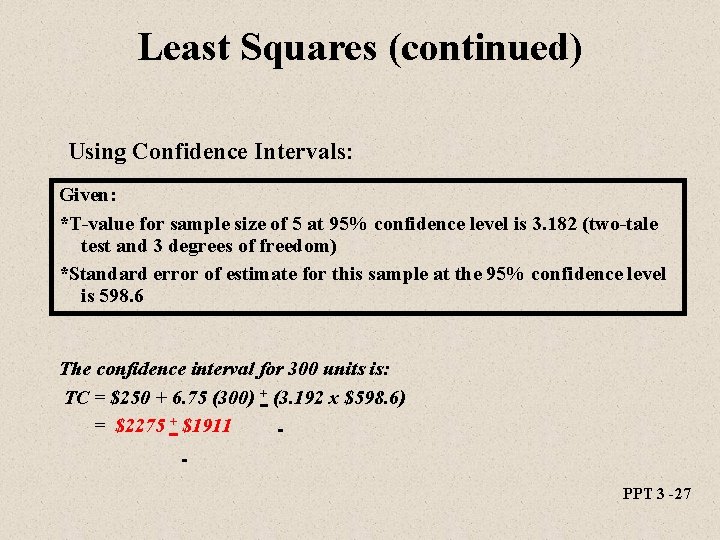
Least Squares (continued) Using Confidence Intervals: Given: *T-value for sample size of 5 at 95% confidence level is 3. 182 (two-tale test and 3 degrees of freedom) *Standard error of estimate for this sample at the 95% confidence level is 598. 6 The confidence interval for 300 units is: TC = $250 + 6. 75 (300) + (3. 192 x $598. 6) = $2275 + $1911 PPT 3 -27

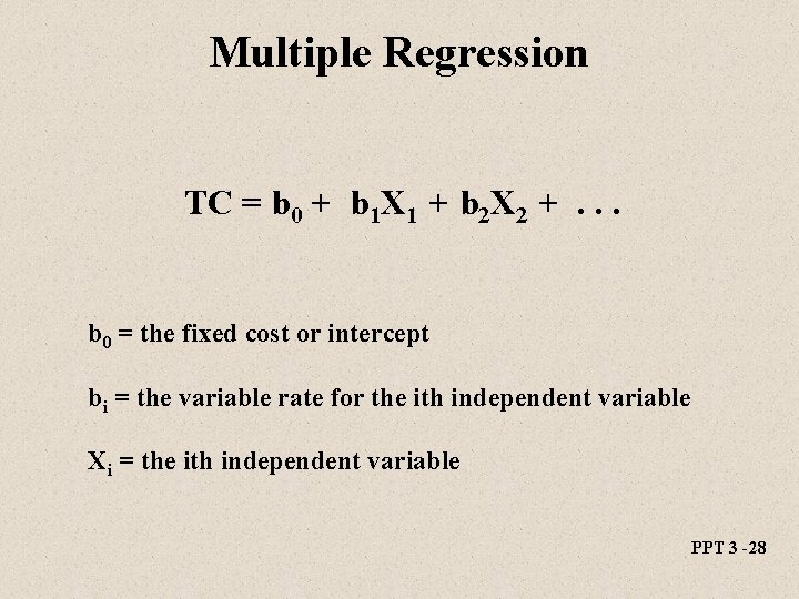
Multiple Regression TC = b 0 + b 1 X 1 + b 2 X 2 +. . . b 0 = the fixed cost or intercept bi = the variable rate for the ith independent variable Xi = the ith independent variable PPT 3 -28

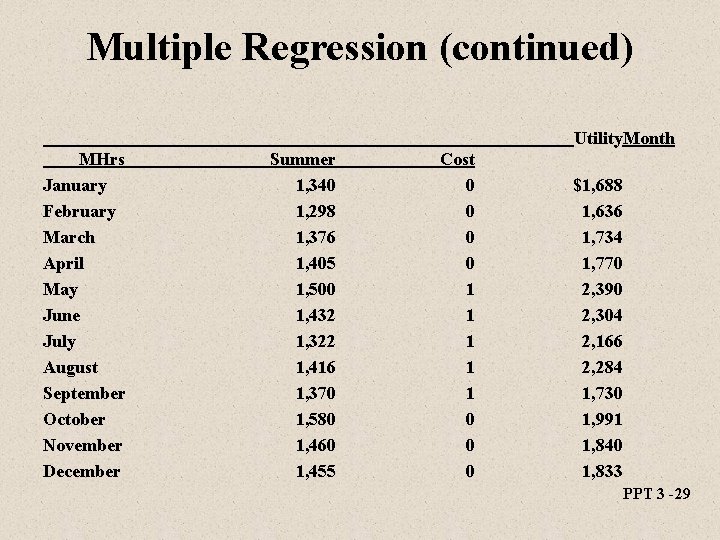
Multiple Regression (continued) Utility. Month MHrs January February March April May June July August September October November December Summer 1, 340 1, 298 1, 376 1, 405 1, 500 1, 432 1, 322 1, 416 1, 370 1, 580 1, 460 1, 455 Cost 0 0 1 1 1 0 0 0 $1, 688 1, 636 1, 734 1, 770 2, 390 2, 304 2, 166 2, 284 1, 730 1, 991 1, 840 1, 833 PPT 3 -29

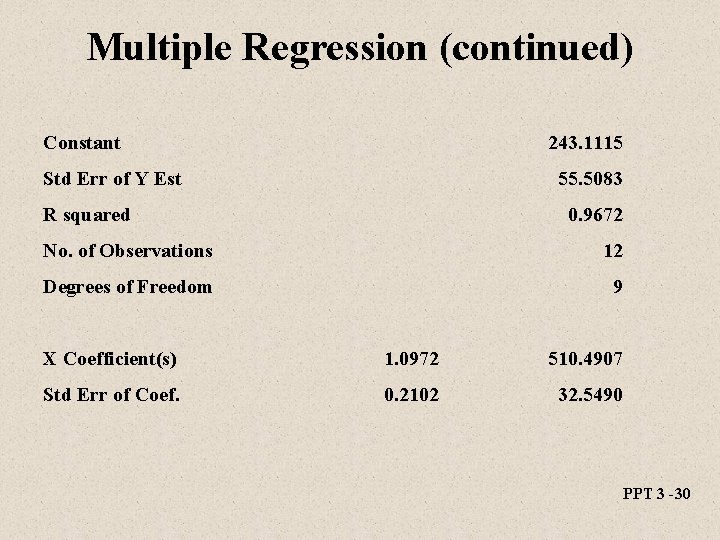
Multiple Regression (continued) Constant 243. 1115 Std Err of Y Est 55. 5083 R squared 0. 9672 No. of Observations 12 Degrees of Freedom 9 X Coefficient(s) 1. 0972 510. 4907 Std Err of Coef. 0. 2102 32. 5490 PPT 3 -30

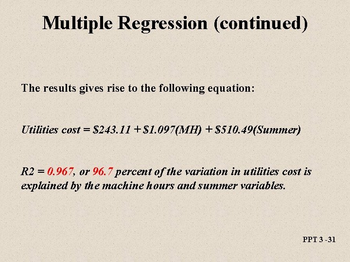
Multiple Regression (continued) The results gives rise to the following equation: Utilities cost = $243. 11 + $1. 097(MH) + $510. 49(Summer) R 2 = 0. 967, or 96. 7 percent of the variation in utilities cost is explained by the machine hours and summer variables. PPT 3 -31

Cost Behavior and Managerial Judgment Some Tips l l l Use past experience Try to confirm results with operating personal Use common sense to confirm statistical studies PPT 3 -32

End of Chapter 3 PPT 3 -33