Fin 501 Asset Pricing Lecture 04 Sharpe Ratio

Fin 501: Asset Pricing Lecture 04: Sharpe Ratio, Bounds and the Equity Premium Puzzle Prof. Markus K. Brunnermeier Lecture 04 Bounds and Equity Premium Puzzle 1

Fin 501: Asset Pricing $1 invested in 1978 - show graph! Lecture 04 Bounds and Equity Premium Puzzle 2

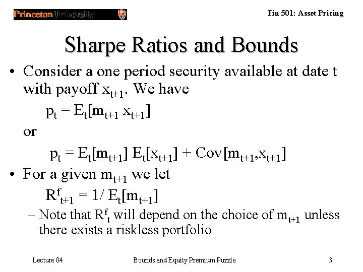
Fin 501: Asset Pricing Sharpe Ratios and Bounds • Consider a one period security available at date t with payoff xt+1. We have pt = Et[mt+1 xt+1] or pt = Et[mt+1] Et[xt+1] + Cov[mt+1, xt+1] • For a given mt+1 we let Rft+1 = 1/ Et[mt+1] – Note that Rft will depend on the choice of mt+1 unless there exists a riskless portfolio Lecture 04 Bounds and Equity Premium Puzzle 3

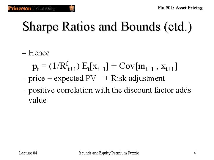
Fin 501: Asset Pricing Sharpe Ratios and Bounds (ctd. ) – Hence pt = (1/Rft+1) Et[xt+1] + Cov[mt+1 , xt+1] – price = expected PV + Risk adjustment – positive correlation with the discount factor adds value Lecture 04 Bounds and Equity Premium Puzzle 4

Fin 501: Asset Pricing in Returns Et [mt+1 xt+1 ] = pt – divide both sides by pt and note that xt+1 = Rt+1 Et [mt+1 Rt+1] = 1 (vector) – using Rft+1 = 1/ Et[mt+1], we get Et [mt+1 (Rt+1 – Rft+1 )] = 0 – m-discounted expected excess return for all assets is zero. Lecture 04 Bounds and Equity Premium Puzzle 5

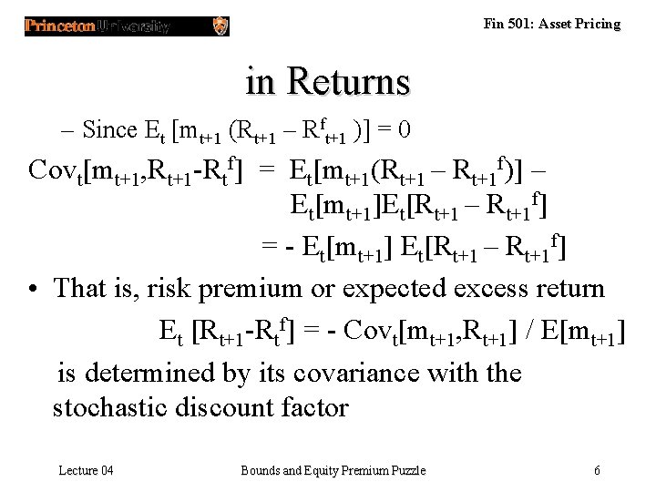
Fin 501: Asset Pricing in Returns – Since Et [mt+1 (Rt+1 – Rft+1 )] = 0 Covt[mt+1, Rt+1 -Rtf] = Et[mt+1(Rt+1 – Rt+1 f)] – Et[mt+1]Et[Rt+1 – Rt+1 f] = - Et[mt+1] Et[Rt+1 – Rt+1 f] • That is, risk premium or expected excess return Et [Rt+1 -Rtf] = - Covt[mt+1, Rt+1] / E[mt+1] is determined by its covariance with the stochastic discount factor Lecture 04 Bounds and Equity Premium Puzzle 6

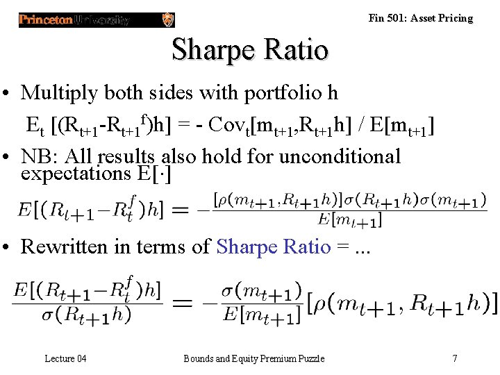
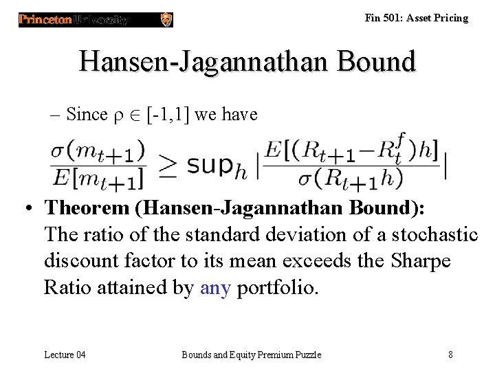
Fin 501: Asset Pricing Sharpe Ratio • Multiply both sides with portfolio h Et [(Rt+1 -Rt+1 f)h] = - Covt[mt+1, Rt+1 h] / E[mt+1] • NB: All results also hold for unconditional expectations E[¢] • Rewritten in terms of Sharpe Ratio =. . . Lecture 04 Bounds and Equity Premium Puzzle 7

Fin 501: Asset Pricing Hansen-Jagannathan Bound – Since r 2 [-1, 1] we have • Theorem (Hansen-Jagannathan Bound): The ratio of the standard deviation of a stochastic discount factor to its mean exceeds the Sharpe Ratio attained by any portfolio. Lecture 04 Bounds and Equity Premium Puzzle 8

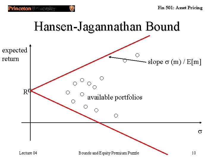
Fin 501: Asset Pricing Hansen-Jagannathan Bound – Theorem (Hansen-Jagannathan Bound): The ratio of the standard deviation of a stochastic discount factor to its mean exceeds the Sharpe Ratio attained by any portfolio. – Can be used to easy check the “viability” of a proposed discount factor – Given a discount factor, this inequality bounds the available risk-return possibilities – The result also holds conditional on date t info Lecture 04 Bounds and Equity Premium Puzzle 9

Fin 501: Asset Pricing Hansen-Jagannathan Bound expected return Rf slope s (m) / E[m] available portfolios s Lecture 04 Bounds and Equity Premium Puzzle 10

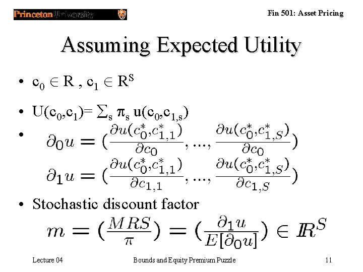
Fin 501: Asset Pricing Assuming Expected Utility • c 0 2 R , c 1 2 RS • U(c 0, c 1)= ås ps u(c 0, c 1, s) • - • Stochastic discount factor Lecture 04 Bounds and Equity Premium Puzzle 11

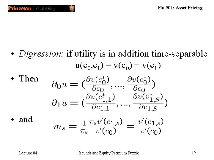
Fin 501: Asset Pricing • Digression: if utility is in addition time-separable u(c 0, c 1) = v(c 0) + v(c 1) • Then • and Lecture 04 Bounds and Equity Premium Puzzle 12

Fin 501: Asset Pricing Equity Premium Puzzle • Recall E[Rj]-Rf = -Rf Cov[m, Rj] • Now: E[Rj]-Rf = -Rf Cov[¶ 1 u, Rj]/E[¶ 0 u] • Recall Hansen-Jaganathan bound Lecture 04 Bounds and Equity Premium Puzzle 13

Fin 501: Asset Pricing Equity Premium Puzzle (ctd. ) u u c 1 c 2 Equity Premium Puzzle: • high observed Sharpe ratio of stock market indices • low volatility of consumption ) (unrealistically) high level of risk aversion Lecture 04 Bounds and Equity Premium Puzzle 14

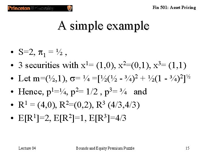
Fin 501: Asset Pricing A simple example • • • S=2, p 1 = ½ , 3 securities with x 1= (1, 0), x 2=(0, 1), x 3= (1, 1) Let m=(½, 1), s= ¼ =[½(½ - ¾)2 + ½(1 - ¾)2]½ Hence, p 1=¼, p 2= 1/2 , p 3= ¾ and R 1 = (4, 0), R 2=(0, 2), R 3 (4/3, 4/3) E[R 1]=2, E[R 2]=1, E[R 3]=4/3 Lecture 04 Bounds and Equity Premium Puzzle 15

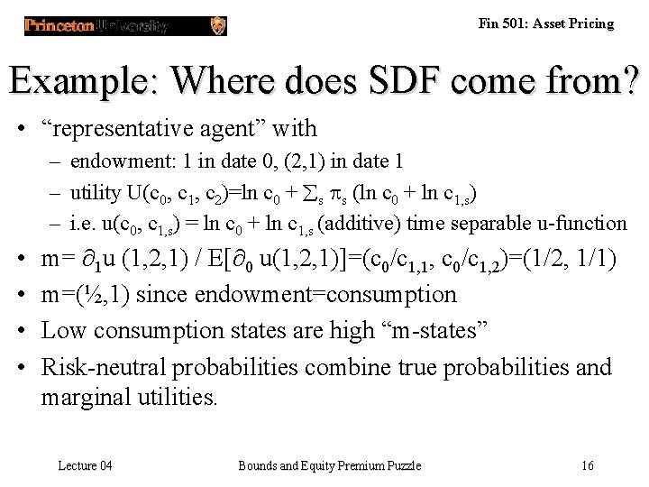
Fin 501: Asset Pricing Example: Where does SDF come from? • “representative agent” with – endowment: 1 in date 0, (2, 1) in date 1 – utility U(c 0, c 1, c 2)=ln c 0 + ås ps (ln c 0 + ln c 1, s) – i. e. u(c 0, c 1, s) = ln c 0 + ln c 1, s (additive) time separable u-function • • m= ¶ 1 u (1, 2, 1) / E[¶ 0 u(1, 2, 1)]=(c 0/c 1, 1, c 0/c 1, 2)=(1/2, 1/1) m=(½, 1) since endowment=consumption Low consumption states are high “m-states” Risk-neutral probabilities combine true probabilities and marginal utilities. Lecture 04 Bounds and Equity Premium Puzzle 16