Bearing Capacity of Shallow Foundation 1 Ultimate Bearing

Bearing Capacity of Shallow Foundation 1

Ultimate Bearing Capacity of Shallow Foundation: To perform satisfactorily, shallow foundations must have two main characteristics: 1. They have to be safe against overall shear failure in the soil that supports them. 2. They cannot undergo excessive or settlement. (The term excessive I relative, because the degree of settlement allowed for a structure depends on several considerations. ) The load per unit area of the foundation at which shear failure in soil occurs is called the ultimate bearing capacity Mode of Bearing Capacity Failures: Bearing capacity failures of foundations can be grouped into three categories 1 - General shear failure. 2 - Local shear failure 3 - punching shear failure 2

A strip foundation with a width of B resting on the surface of a dense sand or stiff cohesive soil, At a certain point when a sudden failure in the soil supporting the foundation will take place, and the failure surface in the soil will extend to the ground surface 3. 1 a. This load per unit area, is usually referred to as the ultimate bearing capacity qu of the foundation. When such sudden failure in soil takes place, it is called general shear failure. If the foundation under consideration rests on sand or clayey soil of medium compaction. A considerable movement of the foundation is required for the failure surface in soil to extend to the ground surface 3. 1 b. The load per unit area at which this happens is the ultimate bearing capacity, qu. Beyond that point, an increase in load will be accompanied by a large increase in foundation settlement. The load per unit area of the foundation, is referred to as the first failure load. Note that a peak value of q is not realized in this type of failure, which is called the local shear failure in soil. If the foundation is supported by a fairly loose soil, the load–settlement plot will be like the one in Figure 3. 1 c. In this case, the failure surface in soil will not extend the ground surface. Beyond the ultimate failure load, the load–settlement plot will be steep and practically linear. This type of failure in soil is called the punching shear failure. 3

The Terzaghi Bearing-Capacity Equation Terzaghi suggested that for a continuous, or strip, foundation (i. e. , one whose width to-length ratio approaches zero), the failure surface in soil at ultimate load may be assumed to be similar to that shown in the Figure. The failure zone under the foundation can be separated into three parts : 1. The triangular zone ACD immediately under the foundation 2. The radial shear zones ADF and CDE, with the curves DE and DF being arcs of a logarithmic spiral 3. Two triangular passive zones AFH and CEG. Figure 3. 3 Bearing capacity failure in soil under a rough rigid continuous (strip) foundation qult = c. Nc+ q. Nq+ 0. 5 g. BNg …. . 3. 1 (For strip footings, such as wall foundations) For (vertical load- no eccentricity – horizontal ground – horizontal base) Where, Nc , Nq and Ng are the soil-bearing capacity factors, dimensionless terms, whose values relate to the angle of internal friction. 4

The bearing capacity factors are defined by ………. 3. 2 ………. . 3. 3 ………. 3. 4 Where the Kpg values and variation of the bearing capacity factors which defined by equations (3. 2), (3. 3) and (3. 4) are given in table (3. 1) qult = 1. 3 c. Nc+ q. Nq+ 0. 4 g. BNg ……. 3. 5 (For square footings, typical of interior columns) qult = 1. 3 c. Nc+ q. Nq+ 0. 3 g. BNg ……. 3. 6 (For circular footings, such as towers, chimneys) In equation (3. 5), B equals to dimension of each side of the foundation in equation (3. 6), B equals the diameter of the foundation. 5

For foundations that exhibit the local shear failure mode in soils, Terzaghi suggested that the following modifications to equations (3. 1), (3. 5) and (3. 6) • 6

Effect of Water Table on Bearing Capacity If the water table is close to the foundation, some modifications of the bearing capacity equations will be necessary. (See the Figure 3. 4) Figure 3. 4 Modification of bearing capacity equations for water table 9

Meyerhof Equation (vertical or inclined load- eccentricity – horizontal ground – horizontal base) qult= c. Nc sc dc+ q Nq sq dq+ 0. 5 B N s d for vertical load qult= c. Nc dc ic+ q Nq dq iq+ 0. 5 B N d i for inclined load 10

Table 3. 2 Bearing-capacity factors for the Meyerhof, Hansen, and Vesic bearing capacity equations 11

Table 3. 3 Shape, depth, and inclination factors for the Meyerhof bearing-capacity equations of Table 3. 2 12

The ultimate bearing capacity for footings with eccentricity, using either the Meyerhof or Hansen equations, is found in either of two ways: Method 1. Use either the Hansen bearing-capacity equation with the following adjustments: a. Use B' in the BN term. b. Use B' and L' in computing the shape factors c. Use actual B and L for all depth factors. The computed ultimate bearing capacity qult is then reduced to an allowable value qall with an appropriate safety factor SF as qall = qult/SF Method 2. Use the Meyerhof general bearing-capacity equation and a reduction factor Re used as qu. It, = qu. It, comp * Re it should be used only with the Meyerhof equation to compute the bearing capacity. The original Meyerhof method gave reduction curves; however, the following equations are suitable for obtaining the reduction factor: Re = 1 - 2 e/B (cohesive soil) Re = 1 – (e/B)1/2 (cohesionless soil and for 0 < e/B < 0. 3) Alternatively, one may directly use the Meyerhof equation with B' and L' used to compute the shape and depth factors and B' used in the 0. 5 g. B'Ng term. 14

Example 3 A footing load test made by a designer produced the following data: D = 0. 5 m B = 0. 5 m L = 2. 0 m 3 g' = 9. 31 k. N/m Ø triaxial= 42. 5° Cohesion c = 0 Pult = 1863 k. N (measured) , qult = 1863/(0. 5 x 2)=1863 k. Pa (computed) Required Compute the ultimate bearing capacity by both Hansen and Meyerhof equations and compare these values with the measured value. Use Hanson equation Since c = 0, any factors with subscript c do not need computing. All g, i and b factors are 1. 00; with these factors identified, the Hansen equation simplifies to qult= q Nq sq dq iq gq bq + 0. 5 B N s d i g b LIB = 2/0. 5 = 4 Øps = 1. 5(42. 5) - 17 = 46. 75° Use Ø = 47° From Hanson equations table 3 -5 for Ø=47 obtain Nq=187 N =299 Calculate s factor sq = 1 + B’/L’ sin Ø eqn. from table 3 -6 =1+ (0. 5/2) sin 47 = 1. 18 sg = 1 - 0. 4 (B’/L’) eqn. from table 3 -6 = 1 - 0. 4 (0. 5/2) = 0. 9 ≥ 0. 6 Calculate d factor k=(D/B) for (D/B)≤ 1 0. 5/0. 5=1 dq= 1+2 tan Ø(1 -sinØ)2 (D/B) = 1+0. 155 (0. 5/0. 5) =1. 155 d =1 for all Ø qult=9. 31(0. 5)(187)(1. 18)(1. 155)+0. 5(9. 31)(0. 5)(299)(0. 9)(1)=1812 k. Pa 15

Using Meyerhof equation By the Meyerhof equations of Table 3 -5 , and Øps= 47°, we can proceed as follows Nq=187 N =(Nq-1)tan(1. 4 Ø) N =(187 -1)tan(1. 4 x 47) =413. 8=414 Kp=tan 2(45+ Ø/2)=6. 44 calculate s factors sq= s = 1+ 0. 1 Kp(B/L) = 1+0. 1( 6. 44)(0. 5/2)=1. 16 calculate d factors 1/2 dq= d = 1+ 0. 1(Kp) (D/B) = 1+0. 1( 2. 54)(0. 5/0. 5)= 1. 25 Substitute into the Meyerhof equation (ignoring any c subscripts): qult= q Nq sq dq+ 0. 5 B N s d qult= 9. 31(0. 5)(187)(l. 16)(1. 25) + 0. 5(9. 31)(0. 5)(414)(1. 16)(1. 25) =2659 k. Pa Example 4 A square footing 1. 8 mx 1. 8 m is loaded with an axial total column load of 1820 k. N at center and Mx=275 k. N. m, My=165 k. N. m. The column size is 0. 4 mx 0. 4 m. Undrained triaxial test give Ø= 36 o and c=9 k. Pa. The foundation base is at 1. 8 m depth the soil has g= 15. 6 k. N/m 3 and the water table is at 6 m depth. What is the allowable gross qall if factor of safety =3 is required against shear failure use: 1 - Hanson B. C equation and the effective area method. 2 - Meyerhof B. C equation and the eccentricity reduction factor. 16

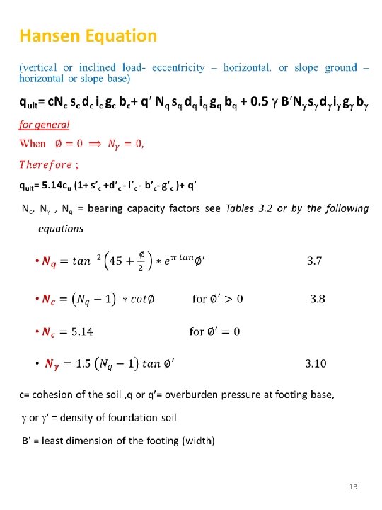
Solution: 1 -Using Hanson BC equation qult= c. Nc sc dc ic gc bc+ q Nq sq dq iq gq bq + 0. 5 B N s d i g b From table 3 -3 for Ø= 36 o Nc=50. 55 Nq= 37. 7 N = 40 Bʹ= B- 2 e L = L- 2 e e. B= 275/1820=0. 15 m e. L= 165/1820=0. 09 m L = 1. 8 - 2 x. 09 = 1. 62 m Bʹ = 1. 8 -2 x 0. 15 = 1. 5 m For h=0 all b factors will equal to 1 For b=0 all g factors will equal to 1 The resultant of all load is vertical so HB and HL =0 all (i) factors are 1 The overburden soil is above W. T eff. = tot. = 15. 6 k. N/m 3 Determine S factors sc= 1+(Nq/Nc). (B’/L’) sc= 1+(37. 7/50. 5)(1. 5/1. 62)=1. 69 sq = 1 + (B’/L’) sin Ø sq= 1+(1. 5/1. 62) sin 36=1. 54 sg = 1 - 0. 4 (B’/L’) =1 -0. 4 (1. 5/1. 62)= 0. 62> 0. 6 determine d factor dc= 1+0. 4 k k= D/B for D/B≤ 1 dc= 1+0. 4 (1. 8/1. 8) = 1. 4 dq= 1+2 tan Ø(1 -sinØ)2 k dq=1+2 tan 36(1 - sin 36)2 1 = 1+0. 247= 1. 247 d =1 for all Ø qult=9(50. 55)(1. 69)(1. 4)+1. 8(15. 6)(37. 7)(1. 54)(1. 247) +0. 5(15. 6)(1. 5)(40)(0. 62)(1) 1076+2033+290=3399 k. Pa Allowable BC qall= 3399/3=1133 k. Pa 17

2 - Meyerhof B. C equation qult= c. Nc sc dc+ q Nq sq dq+ 0. 5 B N s d For Ø = 36 from table 3 -3 Nc=50. 55 Nq=37. 8 N =44. 4 sc= 1+ 0. 2 Kp(B/L) Kp=tan 2(45+ Ø/2)= tan 2(45+18)=3. 84 sc= 1+0. 2(3. 84)(1. 8/1. 8)=1. 77 sq= s = 1+ 0. 1 Kp(B/L) =1+0. 1(3. 84)(1. 8/1. 8)=1. 39 d factor dc = 1+ 0. 2 Kp 1/2 (D/B) 1/2 = 1+ 0. 2 (3. 84) (1. 8/1. 8)= 1. 39 dq= d = 1+ 0. 1 Kp 1/2 (D/B) 1/2 =1+0. 1(3. 84) (1. 8/1. 8)= 1. 2 qult= 9(50. 55)(1. 77)(1. 39) +1. 8(15. 6)(37. 8)(1. 39)(1. 2) +0. 5(15. 6)(1. 8)(44. 4)(1. 39)(1. 2) =1119. 3+1770+1039=3929 k. Pa Allowable BC qall= 3929/3=1309 k. Pa Re. B=1 -(e. B/B)1/2=1 -(0. 15/1. 8)1/2=0. 71 Re. L=1 -(e. L/L)1/2= 1 - (0. 09/1. 8)1/2=0. 77 qall= qall. Re. B. Re. L= 1309(0. 71)(0. 77)= 715. 6 k. Pa 18

Using the Inclination Factors In the general case of inclined loading there is a horizontal component parallel to each base dimension defined as Hi = HB parallel to the B dimension For HB = 0 ; ic, B , iq, B , ig, B are all 1. 0 Hi = HL parallel to the L dimension For HL = 0 ; ic, L , iq, L , ig, L are all 1. 0 These Hi values are used to compute inclination factors for the Hansen equation as follows. dq, B= 1+2 tan Ø(1 -sinØ)2 D/B dq, L= 1+2 tan Ø(1 -sinØ)2 D/L dc, B= 1+0. 4(D/B) dc, L= 1+0. 4(D/L) dc, B= 1+0. 4 tan-1(D/B) dc, L= 1+0. 4 tan-1(D/L) sq, B = 1 + (Bʹ iq, B/L ʹ) sin Ø sq, L = 1 + (Lʹ iq, L/B ʹ) sin Ø sg , B= 1 - 0. 4 (Bʹ ig, B/Lʹ ig, L) sg , L= 1 - 0. 4 (Lʹ ig, L/Bʹ ig, B) sg, I ≥ 0. 6 (if less than 0. 6 use 0. 6) sc, B= 1+(Nq/Nc). (Bʹ ic, B/Lʹ) sc, L= 1+(Nq/Nc). (Bʹ ic, L/Bʹ) ic, B= iq, B-{(1 -iq, B)/(Nq-1)} ic, L= iq, L-{(1 -iq, L)/(Nq-1)} iq, B= {1 - (0. 5 HB)/( V + Af Ca cot Ø)}α 1 iq, L= {1 - (0. 5 HL)/( V + Af Ca cot Ø)}α 1 ig, B= {1 - (0. 7 HB)/( V + Af Ca cot Ø)}α 2 ig, L= {1 - (0. 7 HL)/( V + Af Ca cot Ø)}α 2 These are used in the following modifications of the "edited" Hansen bearing capacity equation qult, B= c. Nc sc, B dc, B ic, B gc, B bc, B + q Nq sq, B dq, B iq, B gq, B bq, B + 0. 5 B N s , B d , B i , B g , B b , B qult, L= c. Nc sc, L dc, L ic, L gc, L bc, L + q Nq sq, L dq, L iq, L gq, L bq, L + 0. 5 L N s , L d , L i , L g , L b , L 19

Example 5 You are given the data shown on the sketch of a load test HL, ult = 382 k. N, Vult = 1060 k. N Required: Find the ultimate bearing capacity by the Hansen method. Øps = 1. 50 Øtri - 17° = 1. 5(43) - 17 = 47. 5° Use Øps = 47°. Nq = 187 Ng = 299 Nc=(Nq-1)cot Ø =(187 -1)cot 47=174 2 tan Ø(1 -sinØ)2 =0. 155 Nq/Nc=187/174=1. 07 All bi = gi = 1. 0 , since both the base and ground are horizontal. dq, B= 1+2 tan Ø(1 -sinØ)2 D/B 1 + 0. 155(0. 5/0. 5) = 1. 16 dq, L= 1+2 tan Ø(1 -sinØ)2 D/L = 1 + 0. 155(0. 5/2. 0) = 1. 04 dg, B = dg, L = 1 iq, B= {1 - (0. 5 HB)/( V + Af Ca cot Ø)}α 1=1 ig, B= {1 - (0. 7 HB)/( V + Af Ca cot Ø)}α 2= 1 iq, L= {1 - (0. 5 HL)/( V + Af Ca cot Ø)}α 1 iq, L= {1 - (0. 5*382)/( 1060 + 0)}2. 5=0. 608 20

ig, L= {1 - (0. 7 HL)/( V + Af Ca cot Ø)}α 2 ig, L= {1 - (0. 7*382)/( 1060 + 0)}2. 5=0. 361 sq, B = 1 + (B’ iq, B/L ’) sin Ø sq, B = 1 + (0. 5*1/2) sin 47=1. 18 sq, L = 1 + (L’ iq, L/B ’) sin Ø sq, L = 1 + (2*0. 608/0. 5) sin 47=2. 78 sg , B= 1 - 0. 4 (B’ ig, B/L’ ig, L) =1 - 0. 4[(0. 5 x l)/(2 x 0. 361)] = 0. 723 > 0. 6 sg , L= 1 - 0. 4 (L’ ig, L/B’ ig, B) = 1 - 0. 4[(2 X 0. 361)/(0. 5 X I)] = 0. 422 < 0. 6 (use 0. 60) qult= c. Nc sc dc ic gc bc+ q Nq sq dq iq gq bq + 0. 5 B N s d i g b qult, B=q Nq sq, B dq, B iq, B + 0. 5 B N s , B d , B i , B = 0. 5(9. 43)(187)(1. 18)(1. 16)(l) + 0. 5(9. 43)(0. 5)(299)(0. 732)(l)(l) = 1206. 9 + 511. 3 = 1718. 2 1700 k. Pa qult, L=q Nq sq, L dq, L iq, L + 0. 5 B N s , L d , L i , L = 0. 5(9. 43)(187)(2. 78)(1. 04)(0. 608) + 0. 5(9. 43)(2. 0)(299)(0. 60)(1. 0)(0. 361) = 1549. 9 + 612. 76 = 2162. 7 215 Ok. Pa Use the smaller computed value, we find the Hansen method seems to give qult = 1700 k. Pa » 106 Ok. Pa of load test. 21