Computer Graphics II Rendering CSE 168 Spr 20

Computer Graphics II: Rendering CSE 168 [Spr 20], Lecture 8: Indirect Lighting Details Ravi Ramamoorthi http: //viscomp. ucsd. edu/classes/cse 168/sp 20

To Do § Homework 2 (Direct Lighting) due Apr 24 § Homework 3 (Path Tracer, Indirect Lighting) May 7 § Assignment is on ed. X edge § START EARLY § This lecture goes through details of indirect lighting, Monte Carlo path tracing for the assignment § Ask re any questions

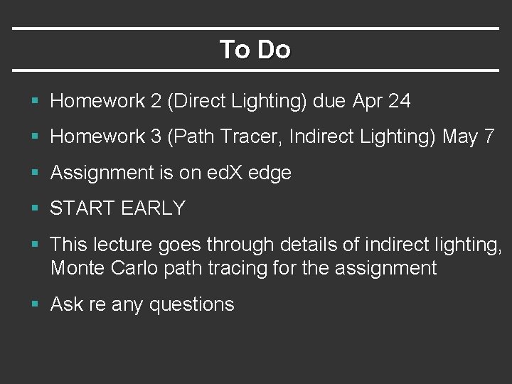
Indirect Lighting § Core of path tracing, global illumination § Supports multiple bounces of light, color bleeding § General paths, general visual effects Light Source (0 bounces) Direct Lighting (1 bounce) Indirect Lighting (2 bounces) Indirect Lighting (3 bounces)

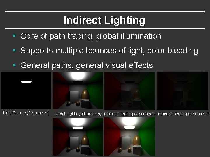
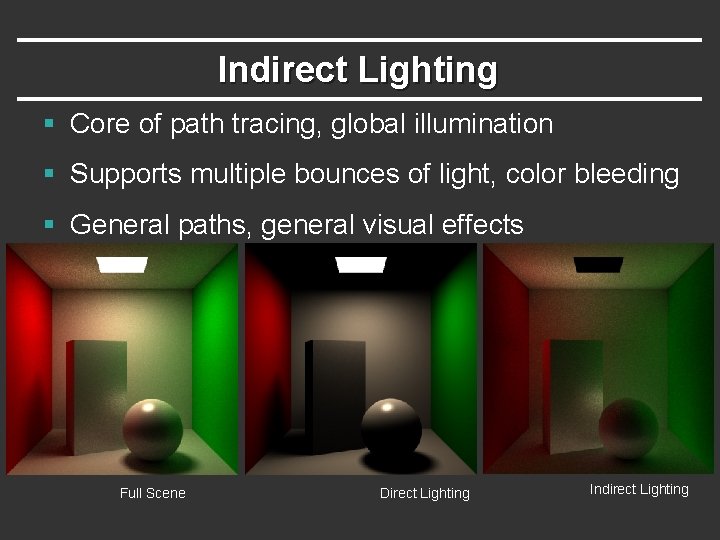
Indirect Lighting § Core of path tracing, global illumination § Supports multiple bounces of light, color bleeding § General paths, general visual effects Full Scene Direct Lighting Indirect Lighting

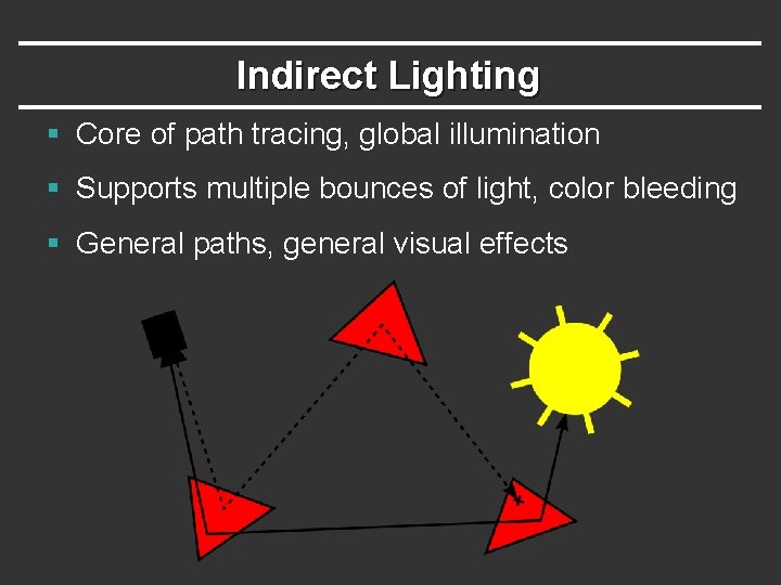
Indirect Lighting § Core of path tracing, global illumination § Supports multiple bounces of light, color bleeding § General paths, general visual effects

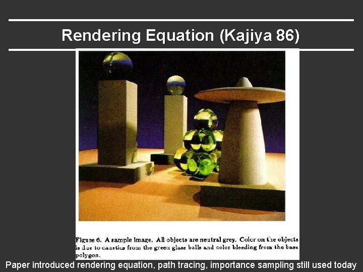
Rendering Equation (Kajiya 86) Paper introduced rendering equation, path tracing, importance sampling still used today

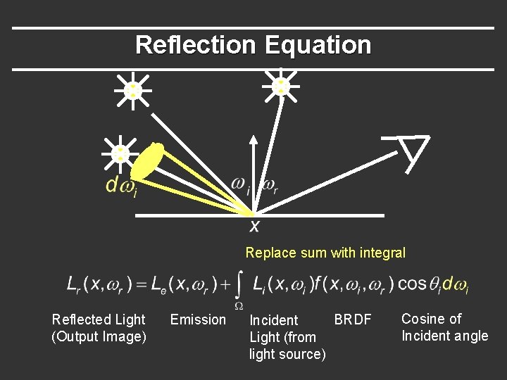
Reflection Equation Replace sum with integral Reflected Light (Output Image) Emission BRDF Incident Light (from light source) Cosine of Incident angle

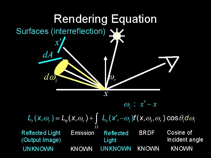
Rendering Equation Surfaces (interreflection) Reflected Light (Output Image) Emission UNKNOWN BRDF Reflected Light UNKNOWN Cosine of Incident angle KNOWN

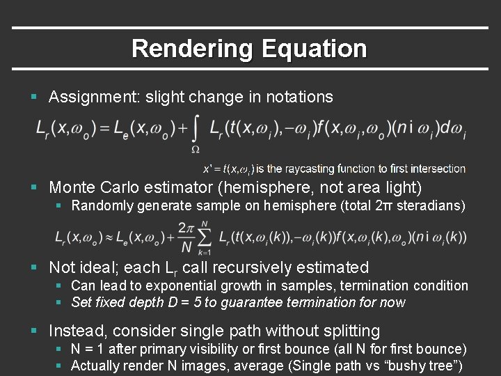
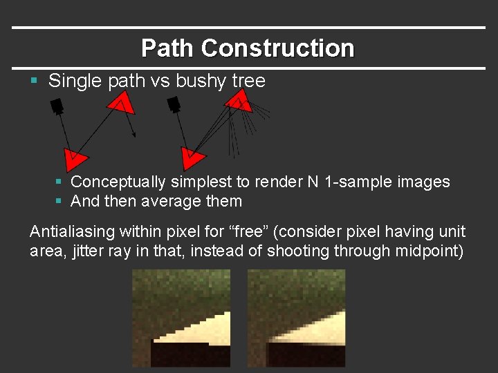
Rendering Equation § Assignment: slight change in notations § Monte Carlo estimator (hemisphere, not area light) § Randomly generate sample on hemisphere (total 2π steradians) § Not ideal; each Lr call recursively estimated § Can lead to exponential growth in samples, termination condition § Set fixed depth D = 5 to guarantee termination for now § Instead, consider single path without splitting § N = 1 after primary visibility or first bounce (all N for first bounce) § Actually render N images, average (Single path vs “bushy tree”)

Path Construction § Single path vs bushy tree § Conceptually simplest to render N 1 -sample images § And then average them Antialiasing within pixel for “free” (consider pixel having unit area, jitter ray in that, instead of shooting through midpoint)

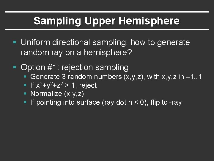
Sampling Upper Hemisphere § Uniform directional sampling: how to generate random ray on a hemisphere? § Option #1: rejection sampling § § Generate 3 random numbers (x, y, z), with x, y, z in – 1. . 1 If x 2+y 2+z 2 > 1, reject Normalize (x, y, z) If pointing into surface (ray dot n < 0), flip to -ray

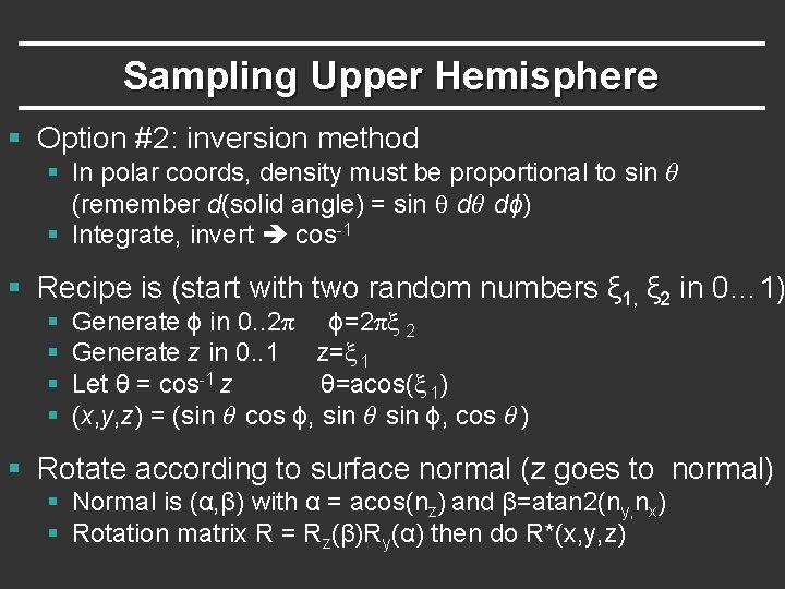
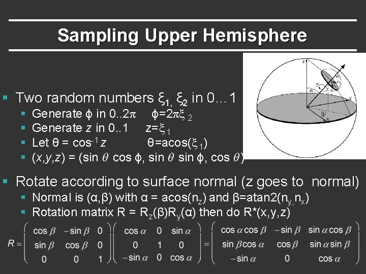
Sampling Upper Hemisphere § Option #2: inversion method § In polar coords, density must be proportional to sin θ (remember d(solid angle) = sin θ dθ dϕ) § Integrate, invert cos-1 § Recipe is (start with two random numbers ξ 1, ξ 2 in 0… 1) § § Generate ϕ in 0. . 2π ϕ=2πξ 2 Generate z in 0. . 1 z=ξ 1 Let θ = cos-1 z θ=acos(ξ 1) (x, y, z) = (sin θ cos ϕ, sin θ sin ϕ, cos θ ) § Rotate according to surface normal (z goes to normal) § Normal is (α, β) with α = acos(nz) and β=atan 2(ny, nx) § Rotation matrix R = Rz(β)Ry(α) then do R*(x, y, z)

Sampling Upper Hemisphere § Two random numbers ξ 1, ξ 2 in 0… 1 § § Generate ϕ in 0. . 2π ϕ=2πξ 2 Generate z in 0. . 1 z=ξ 1 Let θ = cos-1 z θ=acos(ξ 1) (x, y, z) = (sin θ cos ϕ, sin θ sin ϕ, cos θ ) § Rotate according to surface normal (z goes to normal) § Normal is (α, β) with α = acos(nz) and β=atan 2(ny, nx) § Rotation matrix R = Rz(β)Ry(α) then do R*(x, y, z)

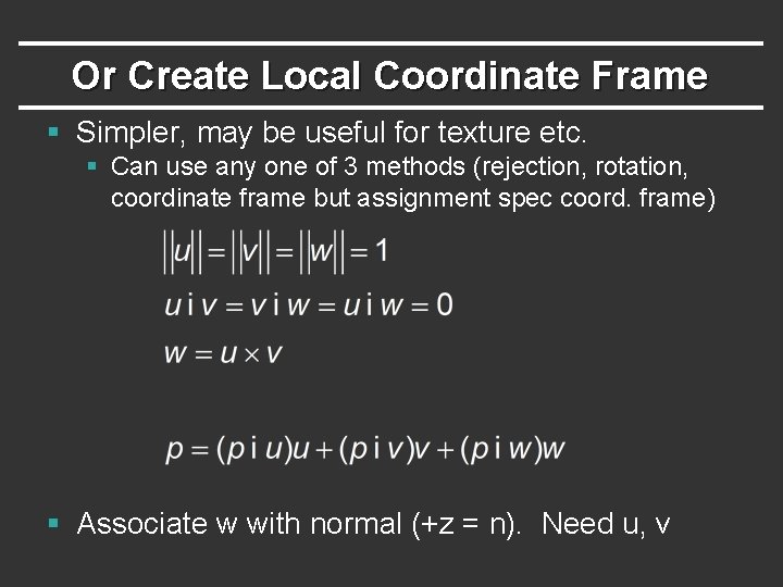
Or Create Local Coordinate Frame § Simpler, may be useful for texture etc. § Can use any one of 3 methods (rejection, rotation, coordinate frame but assignment spec coord. frame) § Associate w with normal (+z = n). Need u, v

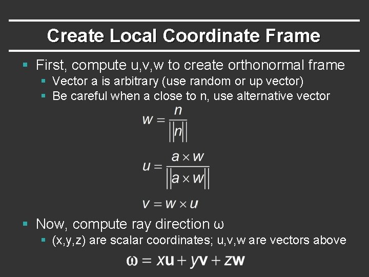
Create Local Coordinate Frame § First, compute u, v, w to create orthonormal frame § Vector a is arbitrary (use random or up vector) § Be careful when a close to n, use alternative vector § Now, compute ray direction ω § (x, y, z) are scalar coordinates; u, v, w are vectors above

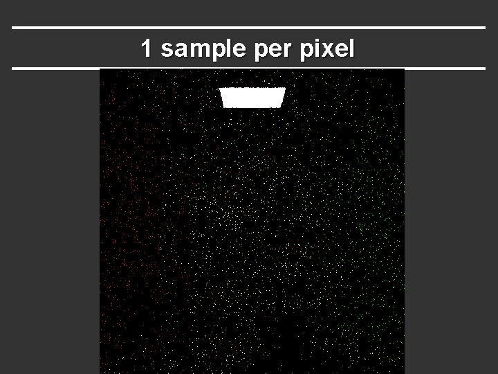
Assignment so far (checkpoint 1) § Sample hemisphere at each bounce § § Evaluate full MC estimator with N = 1 for each ray Upto depth D = 5. Final ray D = 5 returns emit Le only Most rays will actually be 0 (do not hit light source) Very inefficient, but render this, will improve on it next

1 sample per pixel

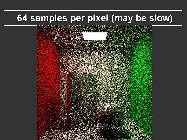
64 samples per pixel (may be slow)

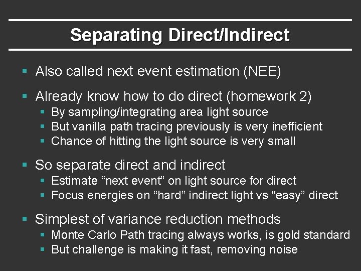
Separating Direct/Indirect § Also called next event estimation (NEE) § Already know how to do direct (homework 2) § By sampling/integrating area light source § But vanilla path tracing previously is very inefficient § Chance of hitting the light source is very small § So separate direct and indirect § Estimate “next event” on light source for direct § Focus energies on “hard” indirect light vs “easy” direct § Simplest of variance reduction methods § Monte Carlo Path tracing always works, is gold standard § But challenge is making it fast, removing noise

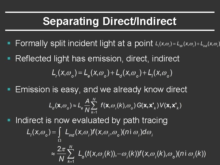
Separating Direct/Indirect § Formally split incident light at a point § Reflected light has emission, direct, indirect § Emission is easy, and we already know direct § Indirect is now evaluated by path tracing

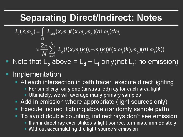
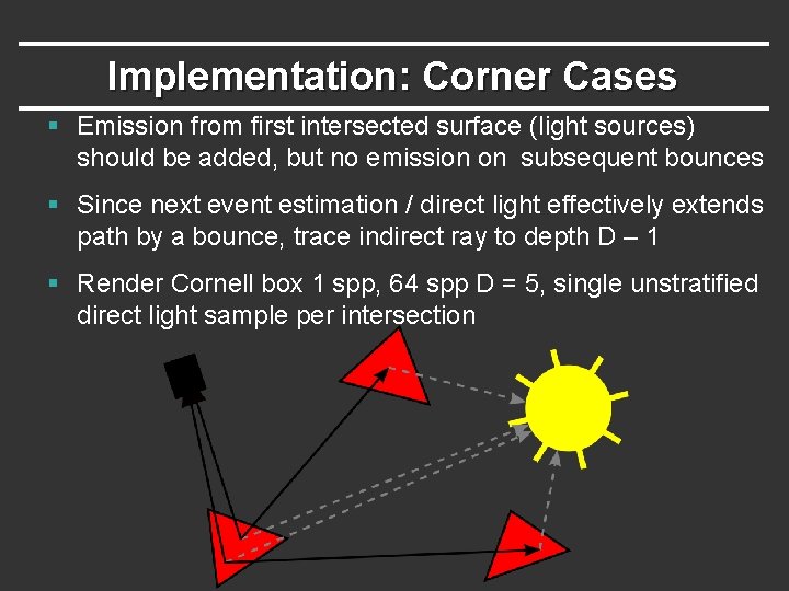
Separating Direct/Indirect: Notes § Note that Lo above = Ld + LI only(not Lr: no emission) § Implementation § At each intersection in path tracer, execute direct lighting § For simplicity, only one (unstratified) ray for each area light § Ultimately, we will average many primary samples § Add in emission where appropriate (light sources only) § Execute indirect lighting above (randomly sample path) § To avoid double counting, indirect rays don’t see emission § If an indirect ray ever strikes a light source, terminate immediately § Without accumulating the light source’s emission

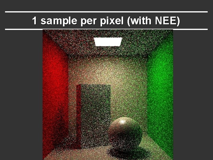
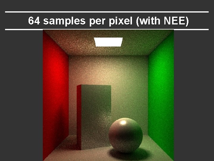
Implementation: Corner Cases § Emission from first intersected surface (light sources) should be added, but no emission on subsequent bounces § Since next event estimation / direct light effectively extends path by a bounce, trace indirect ray to depth D – 1 § Render Cornell box 1 spp, 64 spp D = 5, single unstratified direct light sample per intersection

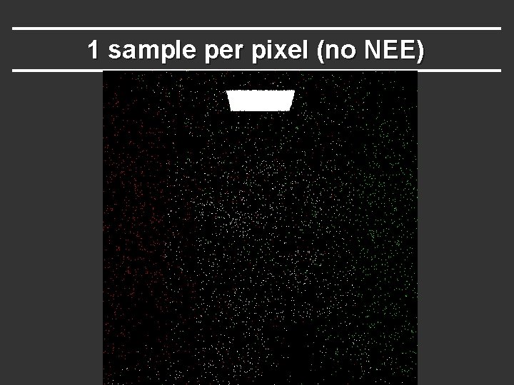
1 sample per pixel (no NEE)

1 sample per pixel (with NEE)

64 samples per pixel (without NEE)

64 samples per pixel (with NEE)

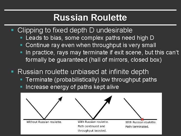
Russian Roulette § Clipping to fixed depth D undesirable § Leads to bias, some complex paths need high D § Continue ray even when throughput is very small § In practice, rays may terminate if exit scene, but this can’t formally be guaranteed (hall of mirrors, closed box) § Russian roulette unbiased at infinite depth § Terminate (probabilistically) low throughput paths § Increase energy of paths kept alive

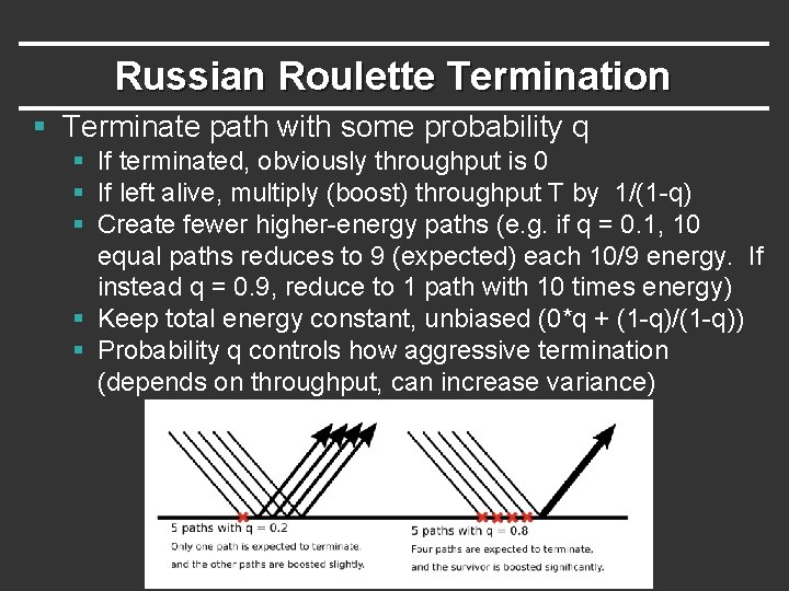
Russian Roulette Termination § Terminate path with some probability q § If terminated, obviously throughput is 0 § If left alive, multiply (boost) throughput T by 1/(1 -q) § Create fewer higher-energy paths (e. g. if q = 0. 1, 10 equal paths reduces to 9 (expected) each 10/9 energy. If instead q = 0. 9, reduce to 1 path with 10 times energy) § Keep total energy constant, unbiased (0*q + (1 -q)/(1 -q)) § Probability q controls how aggressive termination (depends on throughput, can increase variance)

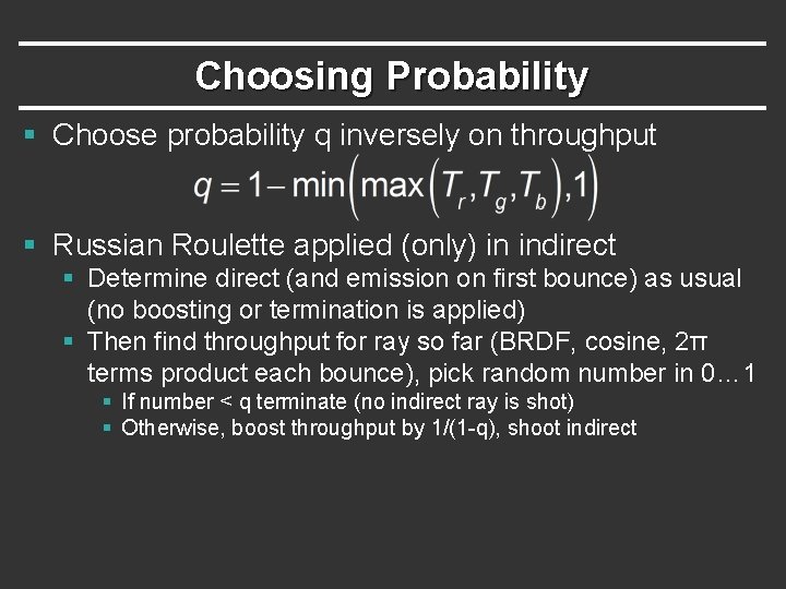
Choosing Probability § Choose probability q inversely on throughput § Russian Roulette applied (only) in indirect § Determine direct (and emission on first bounce) as usual (no boosting or termination is applied) § Then find throughput for ray so far (BRDF, cosine, 2π terms product each bounce), pick random number in 0… 1 § If number < q terminate (no indirect ray is shot) § Otherwise, boost throughput by 1/(1 -q), shoot indirect

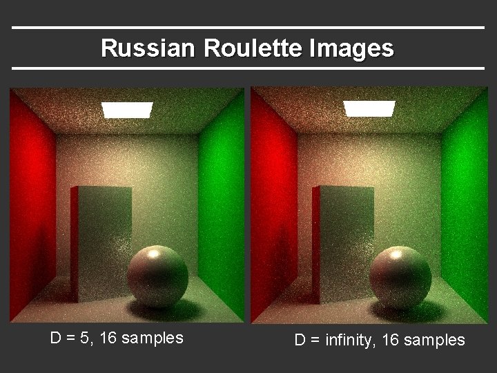
Russian Roulette Images D = 5, 16 samples D = infinity, 16 samples