Common Risk Factors in the Returns on Stocks

Common Risk Factors in the Returns on Stocks and Bonds Eugene F. Fama Kenneth R. French Journal of Financial Economics 1993 Presenter: 周立軒

Brief Saying… • This paper identifies Five common risk factors in the return on stocks and bonds – Two stock market factors, two bond market factors, one market factor. – The five factors seems to explain all returns in stock market and bond market • Except the Low-Grade Bonds

Agenda • • • Introduction The Steps of the Experiment Data & Variables Main Result Conclusion

Introduction • The market βs of Sharpe-Litner, and Breedon’s consumption βs show little relation of the Cross. Sectional average returns on U. S common stocks. • Empirical variables determined average returns are: – Size, Leverage, E/P, BE/ME [Banz(1981), Bhandari(1988), Basu(1983), and Rosenberg, Reid, and Lanstein(1985)]

Introduction • If the market is aggregated, there must be some common factors which can explain both the common stock market and bond market. • But for bond market, the factors used to explain common stock market may not appropriate. – So, the new variables are introduced in this paper

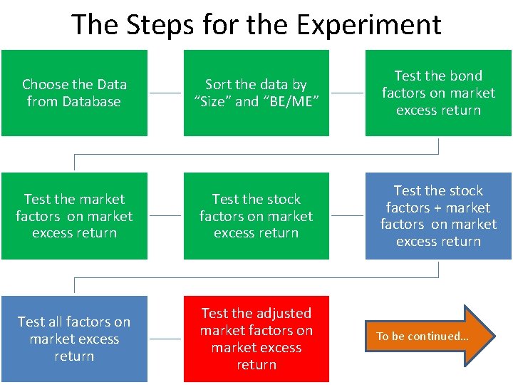
The Steps for the Experiment Choose the Data from Database Sort the data by “Size” and “BE/ME” Test the bond factors on market excess return Test the market factors on market excess return Test the stock factors + market factors on market excess return Test all factors on market excess return Test the adjusted market factors on market excess return To be continued…

Data & Variables • Data – From 1963 to 1991 – At least appeared on COMPUSTAT for two years – Stock price in December on t-1 year and June on t year in CRSP, and book equity in December on t-1 year on COMPUSTAT

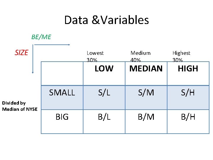
Data &Variables BE/ME SIZE Divided by Median of NYSE Lowest 30% Medium 40% Highest 30% LOW MEDIAN HIGH SMALL S/M S/H BIG B/L B/M B/H

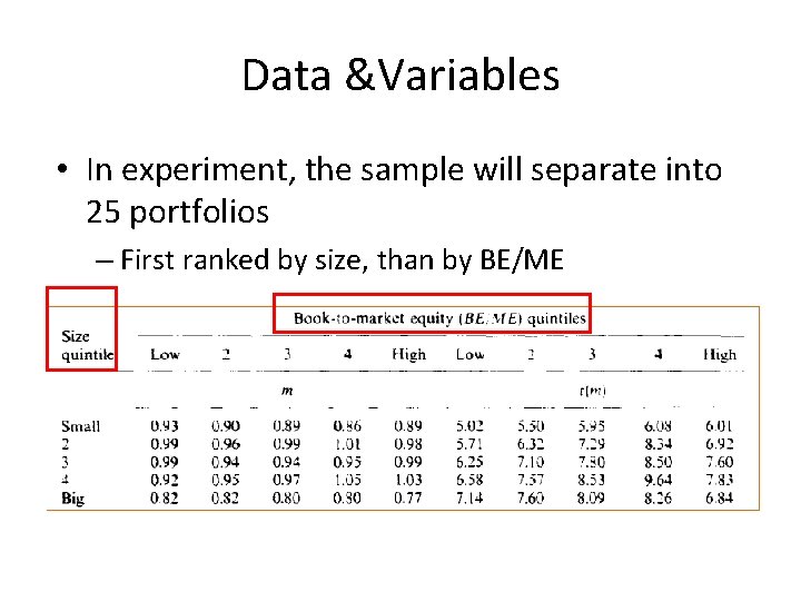
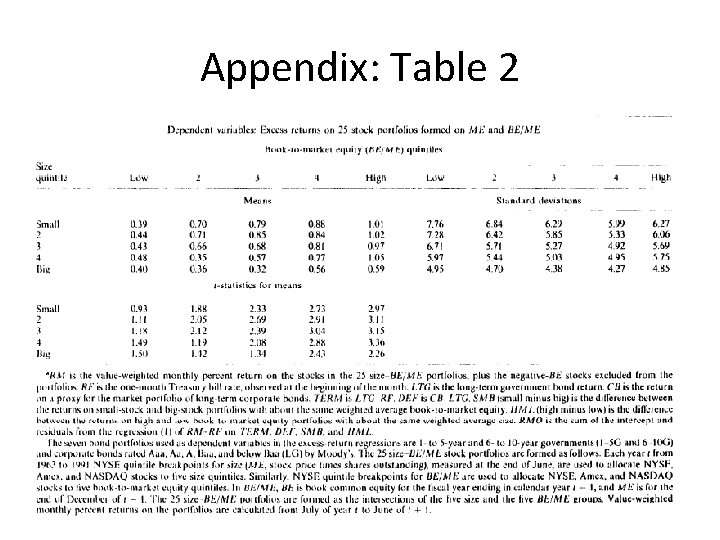
Data &Variables • In experiment, the sample will separate into 25 portfolios – First ranked by size, than by BE/ME

Data & Variables • Why sorting data by SIZE & BE/ME into those number of groups? – The test for these criteria are not sensitive in Fama&French(1992) • After grouping the data, we can start to define the experimental variables

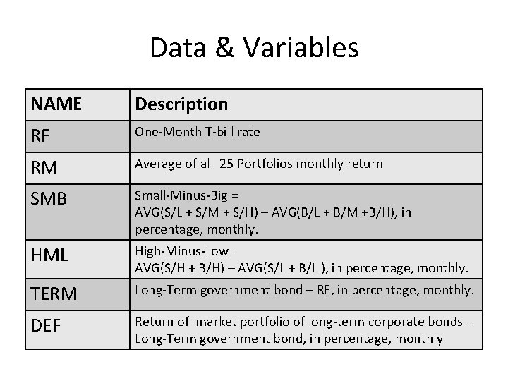
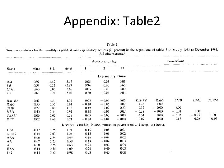
Data & Variables NAME Description RF One-Month T-bill rate RM Average of all 25 Portfolios monthly return SMB Small-Minus-Big = AVG(S/L + S/M + S/H) – AVG(B/L + B/M +B/H), in percentage, monthly. HML High-Minus-Low= AVG(S/H + B/H) – AVG(S/L + B/L ), in percentage, monthly. TERM Long-Term government bond – RF, in percentage, monthly. DEF Return of market portfolio of long-term corporate bonds – Long-Term government bond, in percentage, monthly

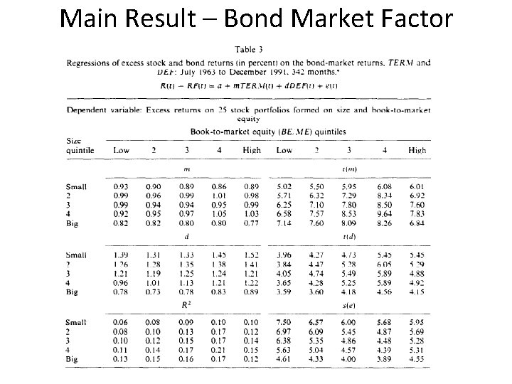
Main Result – Bond Market Factor

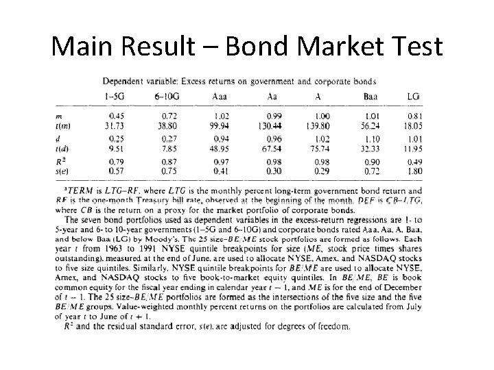
Main Result – Bond Market Test

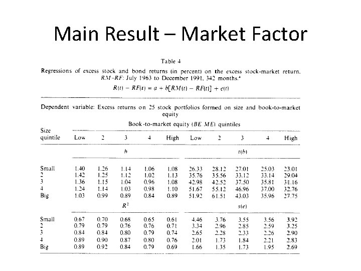
Main Result – Market Factor

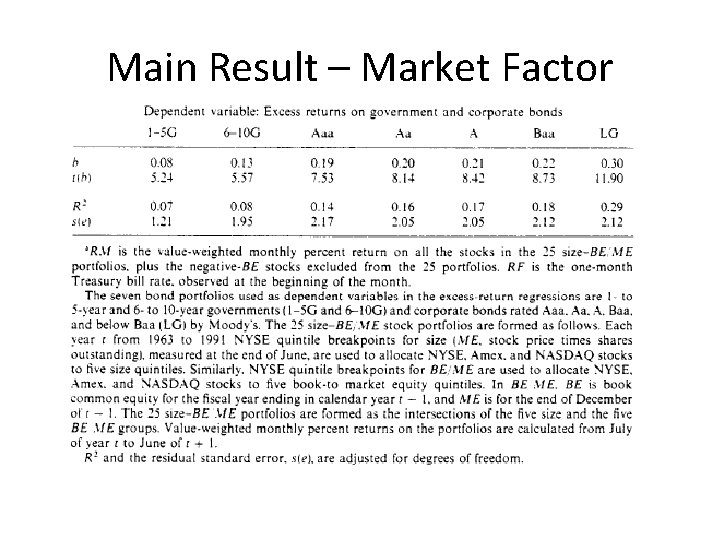
Main Result – Market Factor

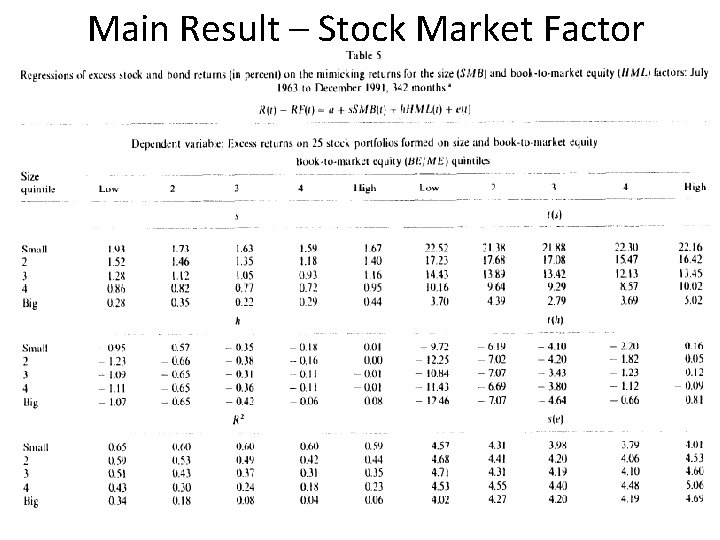
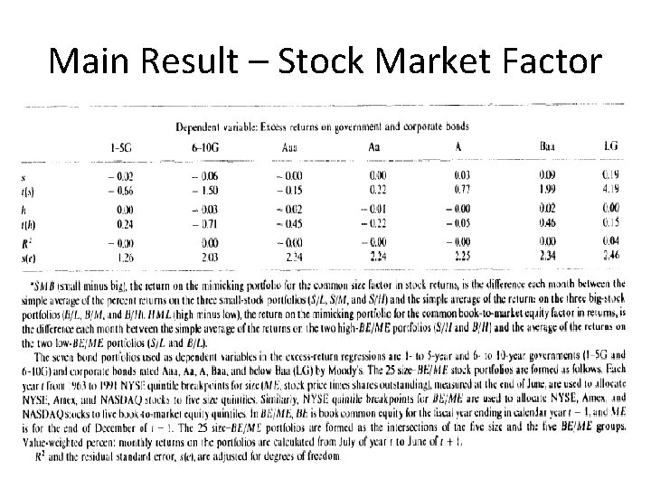
Main Result – Stock Market Factor

Main Result – Stock Market Factor

Main Result – A short break • Even though the market factor, β, seems have explained most part of the variance of stock market, the result still leave room to improve. But , indeed, it capture more common variation for both market. • The bond market factors work well in capturing the common variation of bond market and stock market.

Main Result – A short break • The stock market factors, used alone, cannot explain the variation of bonds well. But they have some ability to explain the variation of stock market. – How about mix the stock market factors with market factor?

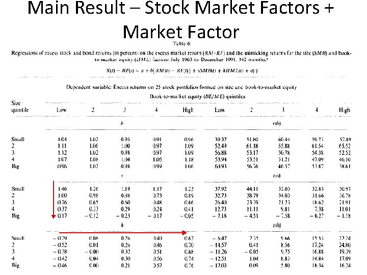
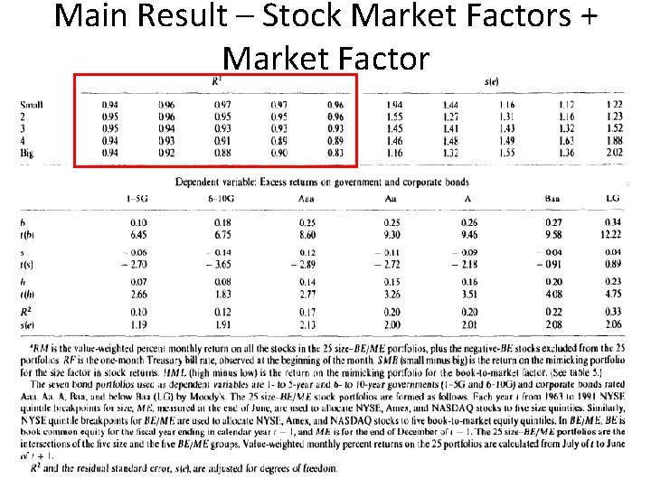
Main Result – Stock Market Factors + Market Factor

Main Result – Stock Market Factors + Market Factor

Main Result • Adding the stock market factors makes the market β move closed to 1. – That’s probably because the RM – Rf have some correlation with HML and SMB. • What if all five factors?

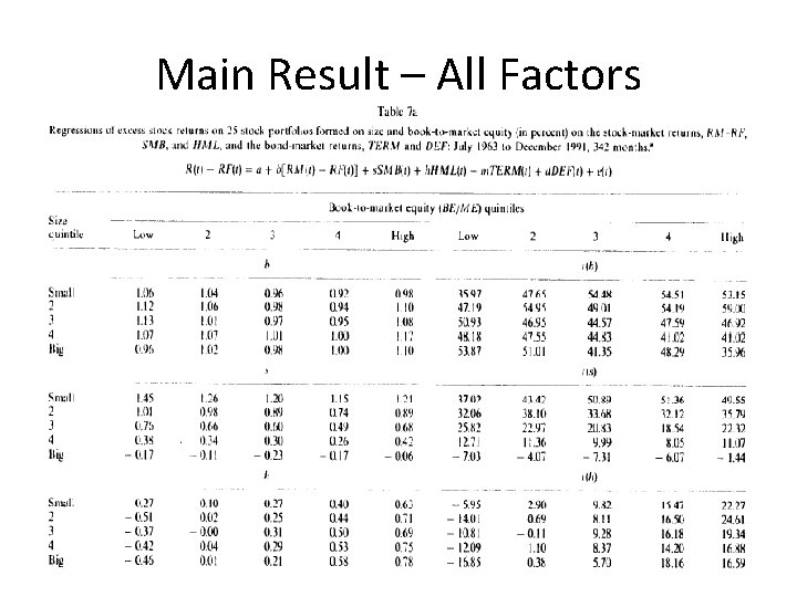
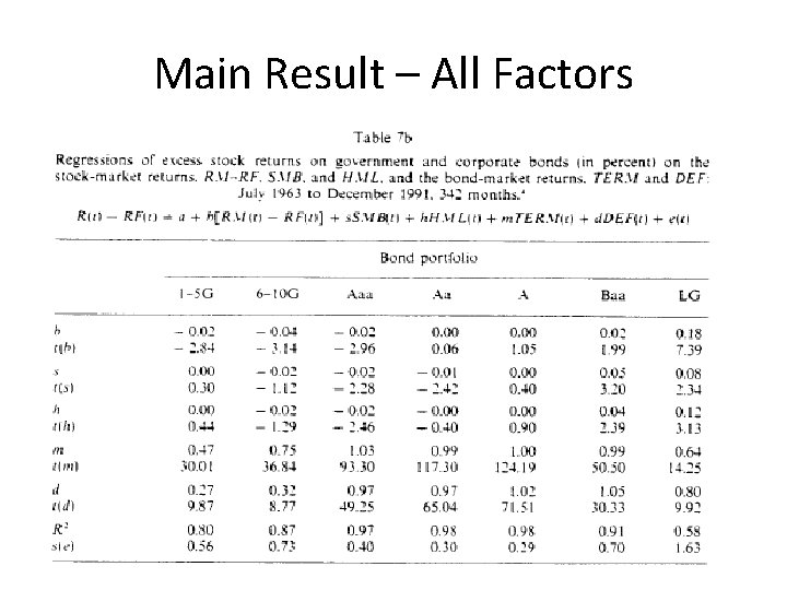
Main Result – All Factors

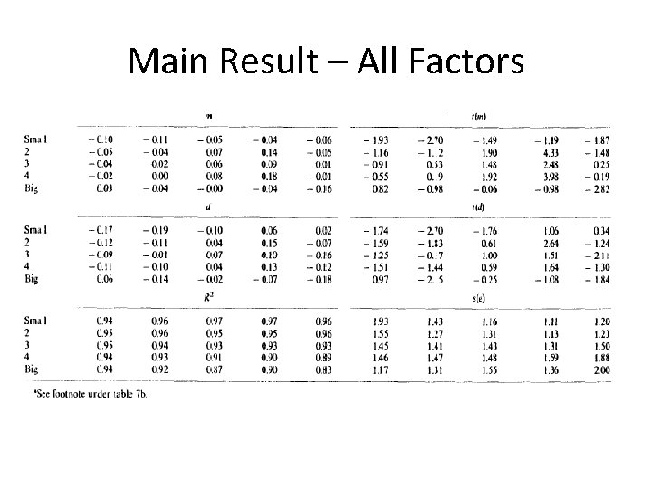
Main Result – All Factors

Main Result – All Factors

Main Result • Five factors regression seems have the contradicted result – The ability of bond market factors for capturing common variation seems lost. – Why? The market factor might be the killer.

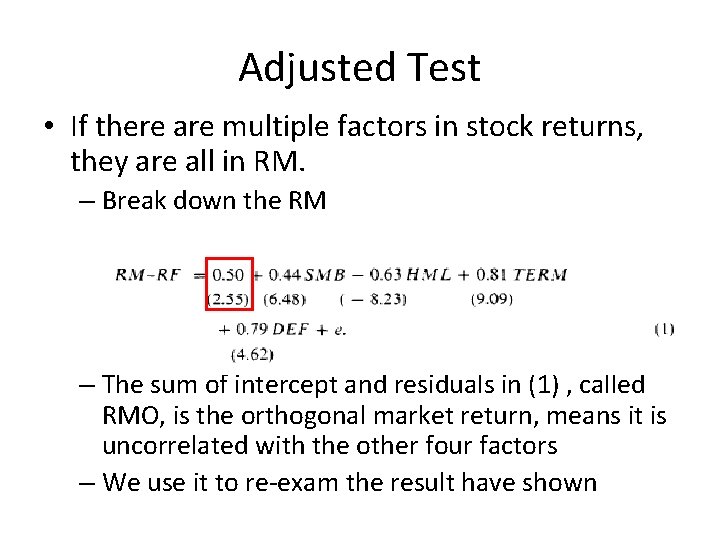
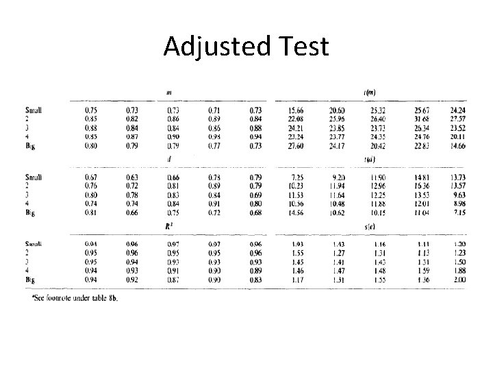
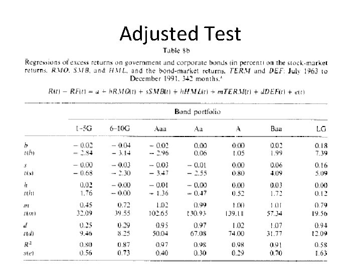
Adjusted Test • If there are multiple factors in stock returns, they are all in RM. – Break down the RM – The sum of intercept and residuals in (1) , called RMO, is the orthogonal market return, means it is uncorrelated with the other four factors – We use it to re-exam the result have shown

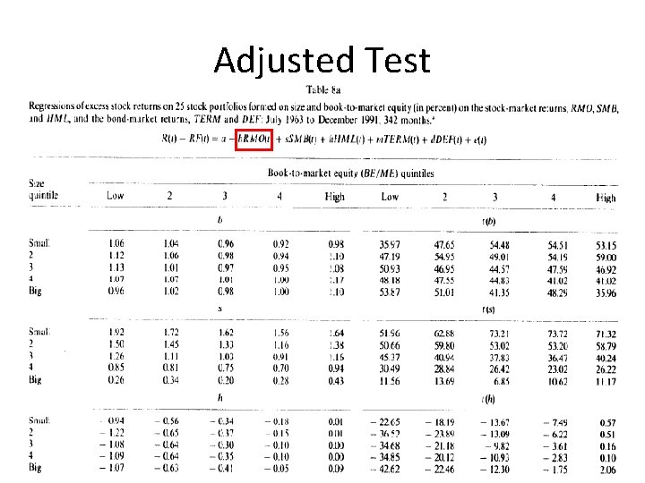
Adjusted Test

Adjusted Test

Adjusted Test

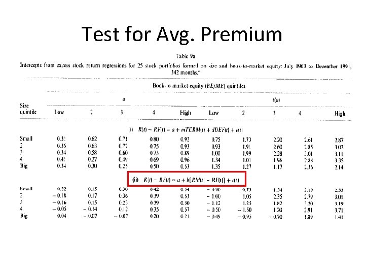
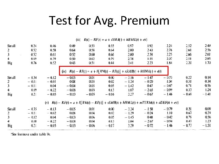
Test for Avg. Premium • In this part, we will test whether the five factors can explain the average premiums on bond and stock markets. • If the five factors are suffice to explain the average returns in market, the intercept should be indistinguishable from 0.

Test for Avg. Premium

Test for Avg. Premium

Test for Avg. Premium

Test for Avg. Premium • The intercept in regression on market factor shows the average premium is affected by SIZE and BE/ME – The market β cannot explain this – But, the market factor is needed to explain why average returns are higher then one-month T-bill rate • In three factor regression, the intercept is closed to 0, this means RM-Rf, HML, SMB can explain the market return well – This is a strong support for Three-Factor Model

Test for Avg. Premium • The TERM and DEF, have little effect on explaining the average premium, although they seem to works well on explaining stock return when used alone. – That may because the average return for TERM and DEF are small, but their high volatility can absorb the common variation well. – So, they can explain the common variation well, but cannot do it as well in average premium

The Bond Market Factors • Do the low premiums of TERM and DEF mean that they are irrelevant with a well-specified asset-pricing model? – Not really, the two factors are affected by business cycle, so, even if the two factors are lack to explain the average premium, they still play a role in model.

Conclusion • The RMO, which is uncorrelated with the other four factors, slopes are all closed to 1 on 25 portfolios, and can be viewed as the premium for being a stock. • The slope for RMO is similar to RM – Rf, so the function of explaining the cross-sectional return are left to SMB and HML • Slope for SMB (in Table 8)can explain why small stock’s returns are much volatilie

Conclusion • As above, the slope for HML can demonstrate the lowest BE/ME portfolio are volatile than the highest BE/ME portfolio – BE/ME is negative correlated with Profitability – The slope for HML can prove this • Five factors do a good job on explaining the whole market’s return – But for evaluating the cross-sectional average stock returns, the three-factor model will be a good alternative

Appendix: Table 2

Appendix: Table 2