Classification Based on lectures by Gideon Dror Isabelle

Classification Based on lectures by Gideon Dror, Isabelle Guyon, and Irit Fishel March 2008

Outline • There are three major learning paradigms, each corresponding to a particular abstract learning task. These are supervised learning, unsupervised learning and reinforcement learning. • We shall focus on classification, which is part of the supervised learning paradigm, providing a comprehensive but intuitive description. In particular: • • • 1. What is classification? 2. Some classification algorithms 3. Dimensional reduction and feature selection 4. Measuring performance 5. Generalization and overfitting 6. Back to Gene Selection in Expression classification

1. The Classification challange Learning of binary classification • Given: a set of m examples (xi, yi) i = 1, 2…m sampled from some distribution D, where xi Rn and yi {-1, +1} • Find: a function f f: Rn -> {-1, +1} which classifies ‘well’ examples xj sampled from D. comments • The function f is usually a statistical model, whose parameters are learnt from the set of examples. • The set of examples are called – ‘training set’. • Y is called – ‘target variable’, or ‘target’. • Examples with yi=+1 are called ‘positive examples’. Examples with yi=-1 are called ‘negative examples’.

Some Real life applications • Systems Biology – Gene expression microarray data: • Text categorization: spam detection • Face detection: Signature recognition: Customer discovery • Medicine: Predict if a patient has heart ischemia by a spectral analysis of his/her ECG.

Microarray data Separate malignant from healthy tissues based on the m. RNA expression profile of the tissue.
 Categorize text documents into predefined categories. For example, categorize news")
Text Categorization (multi category) Categorize text documents into predefined categories. For example, categorize news into ‘sports’, ‘politics’ , ‘science’, etc. Soft tissue found in T-rex fossil Find may reveal details about cells and blood vessels of dinosaurs Health March may be concern when 3: 14 giving Thursday, 24, 2005 Posted: PMkids ESTcell phones Wednesday, (AP) March 23, more 2005 Posted: 11: 14 AMthe EST WASHINGTON -- For than a century, study of SEATTLE, Washington (AP) -- Parents should think twice dinosaurs has beengears limited fossilized bones. Now, Wall Street uptofor jobs before giving in to a middle-schooler's demands for a cell researchers have March recovered 70 -million-year-old Saturday, 26, 2005: 11: 41 AM EST soft tissue, phone, some because potential including what mayscientists be bloodsay, vessels and cells, fromlong-term a health risks remain unclear. finds atmosphere on Saturn Tyrannosaurus rex. (CNN/Money) NEWProbe YORK - Investors onmoon Inflation Watch 2005 Thursday, March 17, 2005 Posted: 11: 17 AM EST have a big week to look forward to -- or be wary of -LOS ANGELES, California -- The space probe depending on how you look at (Reuters) it. Cassini discovered a significant atmosphere around Saturn's moon Enceladus during two recent passes close by, the Jet Propulsion Laboratory said on Wednesday

Face detection • discriminating human faces from non faces.

Signature recognition • Recognize signatures by structural similarities which are difficult to quantify. • does a signature belongs to a specific person, say Tony Blair, or not.

Cusomer discovery • predict whether a customer is likely to purchase certain goods according to a database of customer profiles and their history of shopping activities.
 • Identify handwritten characters: classify each image of character into")
Character recognition (multi category) • Identify handwritten characters: classify each image of character into one of 10 categories ‘ 0’, ‘ 1’, ‘ 2’ … 6132 2056 2014 4283 2064

Classification problem x 2 ? ? ? ? x 1

Classification algorithms – – – – Fisher linear discriminant KNN Decision tree Neural networks SVM Naïve bayes Adaboost Many more …. – Each one has its properties wrt bias, speed, accuracy, transparency…

No Free Lunch Theorem There is a lack of inherent superiority of any classifier • If we make no prior assumption about the nature of the classification task, is any classification method superior overall? • Is any algorithm overall superior to random guessing? • Answer is No to both questions. .

No Free Lunch Theorem Learning algorithm 1 is better than learning algorithm 2 are ultimately statements about the relevant target functions • Experience with a broad range of techniques is the best insurance for solving arbitrary new classification problems

Ugly Duckling Theorem • No-Free Lunch addresses learning or classification. • In the absence of assumptions there is no “best” feature representation.

Fisher Linear Discriminant A classification method that projects high-dimensional data onto a line and performs classification in this one-dimensional space. – Find the direction w that maximizes the distance between the means of the two classes while minimizing the variance within each class. x 2 -No hyperparameters But reduction to 1 D. . The solution involves the inverse of a covariance-like matrix. Related to PCA and linear perceptrons. w ? ? ? ? x 1

KNN – K nearest neighbors – Find the k nearest neighbors of the test example , and infer its class using their known class. – E. g. K=3 x 2 ? ? ? ? ? x 1

KNN – properties • Lazy learning - where the function is only approximated locally and all computation is deferred until classification. • Has a weighted version, and can also be used for regression. • Usually works very well when there is a natral ‘distance’ between examples (Euclidean, Manhattan). • In case the training set is large (say 10^6 examples), and the calculation of distance is non-trivial - could be very slow. • Only a single hyper-parameter – K (usually optimized using cross-validation).

Decision tree – leaves represent classifications and branches represent tests on features that lead to those classifications x 2 ? X 1 > 1 2 NO YES ? ? X 2 > 2 YES NO ? 1 x 1
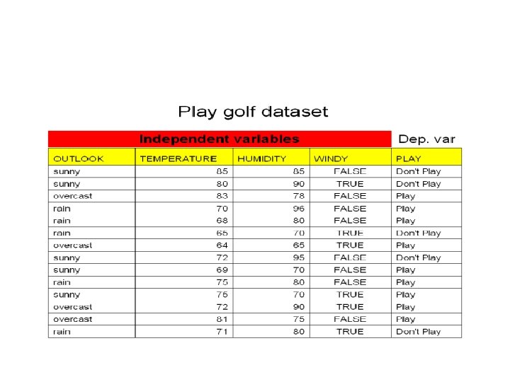
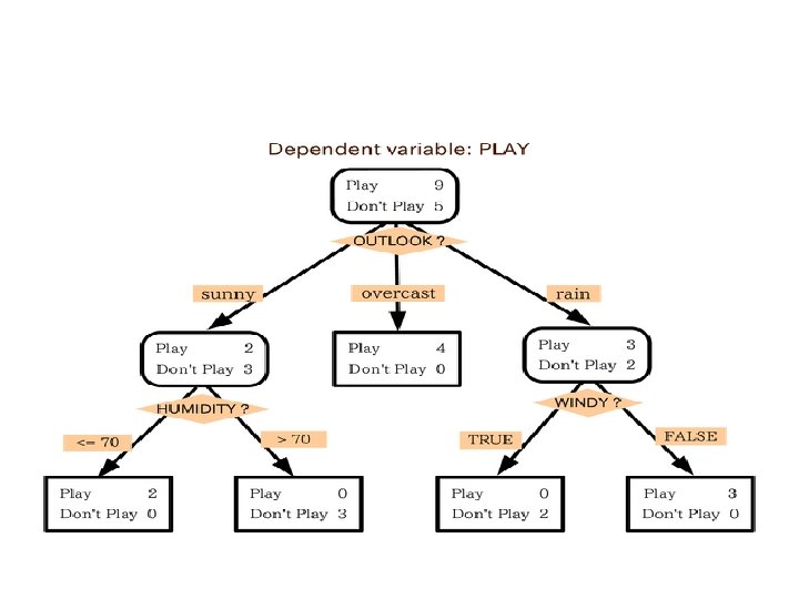

Decision tree learning • The problm of building the most compact tree compatible with training examples is NP complete. • Many heuristic methods for constructiong ‘good’ trees. ID 3, C 4. 5, CART … • Most methods use some greedy manner (find the feature that best divides positive examples from negative examples etc -- Information gain) • One of the simplest algorithms – no hyperparameters. • Outcome is transparent to the user! • Able to handle both numerical and categorical data • Robust, performs well with large data in a short time

Neural network – Find the best separating plane between two classes. – Find an optimal curve separating the two classes. x 2 ? ? – Complicated structure, with many parameters and several hyperparameters, non – trivial to tune. – Prone to overfitting. ? ? x 1

Properties of NNs • • • A clear biological analogy/motivation. The Perceptron is a linear classifier for classifying data specified by an output function f = w'x + b. Its parameters are adapted with an ad-hoc rule similar to stochastic steepest gradient descent. The Perceptron can only perfectly classify a set of data which is linearly separable. The rediscovery of the backpropagation algorithm was probably the main reason behind the repopularization of neural networks, and the introduction of learning multilayered sigmoidal networks, MLPs (where each node has an activation function f = g(w'x + b)) for classification and regression. Backpropagation: The employment of the chain rule of differentiation in deriving the appropriate parameter updates results in an algorithm that `backpropagates’ the errors during training. It is essentially a form of gradient descent. steepest gradient descent methods cannot be relied upon to give the solution without a good starting point. Could such learning be implemented in the brain ? !?

2. Dimensionality reduction -- motivation – May Improve performance of classification algorithm by removing irrelevant features - Defying the curse of dimensionality - simpler models result in – improved generalization: [ The curse of dimensionality: the exponential increase in volume – associated with adding extra dimensions to a space. For example, 100 evenly -spaced sample points suffice to sample a unit interval with no more than 0. 01 distance between points; an equivalent sampling of a 10 -dimensional unit hypercube with a spacing of 0. 01 between adjacent points would require 10^20 sample points: thus, the 10 -dimensional hypercube can be said to be a factor of 10^18 "larger" than the unit interval. Hence, in the context of classification/function approximation. . ] – Classification algorithm may not scale up to the size of the full feature set either in space or time – Allows us to better understand the domain – Cheaper to collect and store data based on reduced feature set.

Two approaches for dimensionality reduction – Feature construction – Feature selection
 Feature construction • Linear methods – – Principal component analysis (PCA) Independent component")
(a) Feature construction • Linear methods – – Principal component analysis (PCA) Independent component analysis (ICA) Fisher linear discriminant …. – – Non linear component analysis (NLCA) Kernel PCA Local linear embedding (LLE) …. • Non-linear methods
 (1) • PCA is mostly used as a tool in")
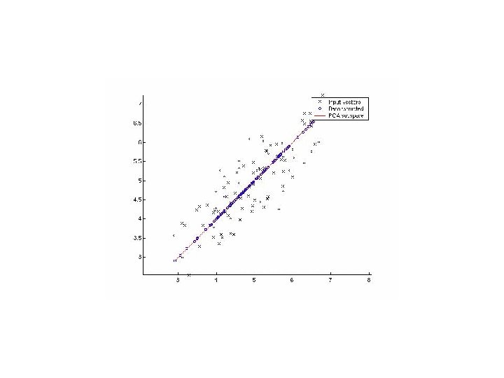
Principal component analysis (PCA) (1) • PCA is mostly used as a tool in exploratory data analysis and for making predictive models. • PCA involves the calculation of the eigenvalue decomposition of a data covariance matrix, usually after mean centering the data for each attribute. • PCA is mathematically defined as an orthogonal linear transformation that transforms the data to a new coordinate system such that the greatest variance by any projection of the data comes to lie on the first coordinate (called the first principal component), the second greatest variance on the second coordinate, and so on. • PCA is theoretically the optimal linear scheme, in terms of least mean square error, for compressing a set of high dimensional vectors into a set of lower dimensional vectors and then reconstructing the original set.
 (2) • The applicability of PCA is limited by the")
Principal component analysis (PCA) (2) • The applicability of PCA is limited by the assumptions made in its derivation: • 1. Linearity: We assume the observed data set are linear combinations of certain basis vectors. • 2. PCA only finds the independent axes of the data under the Gaussian assumption. • 3. It is only when we believe that the observed data has a high signal-to-noise ratio that the principal components with larger variance correspond to interesting dynamics and lower ones correspond to noise.
 Feature selection • Given examples (xi, yi) where xi Rn, select a minimal")
(b) Feature selection • Given examples (xi, yi) where xi Rn, select a minimal subset of features which maximizes the performance, e. g. accuracy. • Exhaustive search is computationally prohibitive, except for a small number of dimensions -- there are O(2 n) possible combinations. • Basically it is an optimization problem, where the classification error is the function to be minimized. But due to the size of search space, heuristics are used.

Filters, Wrappers, and Embedded methods All features Filter Feature subset Multiple Feature subsets Predictor Wrapper All features Embedded method Feature subset Predictor

Filtering – Order all features according to strength of association with the target yi – Various measures of association may be used: • • • Pearson correlation R(Xi) = cov(Xi, Y)/ Xi Y 2 (discrete variables Xi) Fisher Criterion Scoring F(Xi) = | +Xi- -Xi| / ( +Xi 2+ -Xi 2) Golub criterion F(Xi) = | +Xi- -Xi| / | +Xi+ -Xi| Mutual information I(Xi, Y) = p(Xi, Y) log(p(Xi, Y)/p(Xni)p(Y) • … – Choose the first k features and feed them to the classifier

Filtering - characteristics – Usually works well when features are independent, since each feature is considered in isolation. – When the dependencies between features and the targets are important – filtering will not perform very well. • For example, with the XOR problem – Estimated independently of classifier – Still, on many problems filtering is very effective – are relatively robust to overfitting.

Leukemia Diagnosis n’ -1 +1 +1 -1 m {-yi} Golub et al, Science Vol 286: 15 Oct. 1999 {yi}, i=1: m

Prostate Cancer Genes HOXC 8 G 4 G 3 BPH RACH 1 U 29589 RFE SVM, Guyon-Weston, 2000. US patent 7, 117, 188 Application to prostate cancer. Elisseeff-Weston, 2001

RFE SVM for cancer diagnosis Differenciation of 14 tumors. Ramaswamy et al, PNAS, 2001
 - 2543 compounds tested for")
QSAR: Drug Screening Binding to Thrombin (Du. Pont Pharmaceuticals) - 2543 compounds tested for their ability to bind to a target site on thrombin, a key receptor in blood clotting; 192 “active” (bind well); the rest “inactive”. Training set (1909 compounds) more depleted in active compounds. - 139, 351 binary features, which describe three-dimensional properties of the molecule. Number of features Weston et al, Bioinformatics, 2002

Wrappers Use the classifier as a black box, to search in the space of feature subsets, the subset which maximizes classification accuracy. Search is exponentially hard. A common example of heuristic search is hill climbing: keep adding features one at a time until no further improvement can be achieved (“forward selection”) Alternatively we can start with the full set of predictors and keep removing features one at a time until no further improvement can be achieved (“backward selection”)

Embedded methods: Recursive Feature Elimination - RFE 0. Set V = n (total number of features) 1. build linear Support Vector Machine classifiers using V features 2. compute weight vector w = iyixi of optimal hyperplane. Omit V/2 features with lowest |wi|. 3. repeat steps 1 and 2 until one feature is left 4. choose the feature subset that gives the best performance (using cross-validation) (Has strong theoretical justification – tractable and less prone to over fitting – the best of both worlds. . )
 • • • Precision and Recall are two widely")
Measures of classification performance (1) • • • Precision and Recall are two widely used measures for evaluating classification performance. Precision can be seen as a measure of exactness or fidelity, whereas Recall is a measure of completeness. Precision for a class is the number of true positives (i. e. the number of items correctly labeled as belonging to the class) divided by the total number of elements labeled as belonging to the class - TP/(TP+FP). Recall is the number of true positives divided by the total number of elements that actually belong to the class – TP/(TP+FN). A Precision score of 1. 0 for a class C means that every item labeled as belonging to class C does indeed belong to class C (but says nothing about the number of items from class C that were not labeled correctly) whereas a Recall of 1. 0 means that every item from class C was labeled as belonging to class C (but says nothing about how many other items were incorrectly also labeled as belonging to class C). - as we shall see: (a) – there is a threshold dependent tradeoff, and (b) – an integrated measure is hence needed.
 • • • A popular measure that combines Precision")
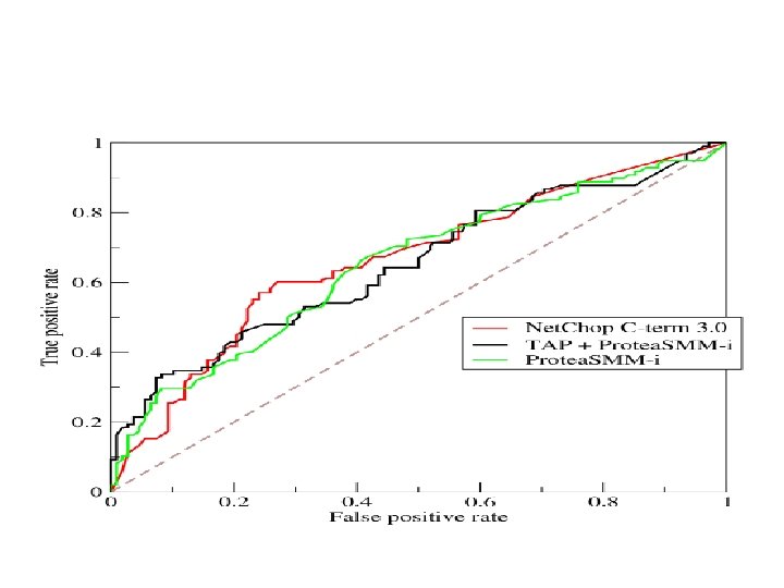
Measures of classification performance (2) • • • A popular measure that combines Precision and Recall is the weighted harmonic mean of precision and recall, the traditional Fmeasure or balanced F-score: F = 2(Px. R)/(P+R) Define the True positive rate as TPR = TP / P = TP / (TP + FN) Define the False positive rate as FPR = FP / N = FP / (FP + TN) A receiver operating characteristic (ROC), or simply ROC curve, is a graphical plot of TPR vs FPR for a binary classifier system as its discrimination threshold is varied. The AUC is equal to the probability that a classifier will rank a randomly chosen positive instance higher than a randomly chosen negative one.
 • Resubstitution estimation: error rate on the learning set – Problem:")
Performance assessment (I) • Resubstitution estimation: error rate on the learning set – Problem: downward bias • Test set estimation: divide cases in learning set into two sets, L 1 and L 2; classifier built using L 1, error rate computed for L 2. L 1 and L 2 must be iid. – Problem: reduced effective sample size
 • m-fold cross-validation (CV) estimation: Cases in learning set randomly divided")
Performance assessment (II) • m-fold cross-validation (CV) estimation: Cases in learning set randomly divided into m subsets of (nearly) equal size. Build classifiers leaving one set out; test set error rates computed on left out set and averaged. • Very popular method. • Is typically used also for tuning hyperparameters.
 • Common error to do feature selection using all of the")
Performance assessment (III) • Common error to do feature selection using all of the data, then CV only for model building and classification • However, usually features are unknown and the intended inference includes feature selection. Then, CV estimates as above tend to be downward biased. • Features should be selected only from the learning set used to build the model (and not the entire learning set)

Generalization and overfitting x 2 ? ? ? ? x 1

Control on the complexity of the model Regularization is intended to reduce the complexity of the model in order to have better generalization • Regularization in decision trees (pruning, ensembling) • Regularization in neural networks (penalty term) • Regularization in SVM

Meta Analysis of Gene Expression Data: A Predictor-Based Approach By Irit Fishel Joint work with: Alon Kaufman Eytan Ruppin

Potential Application of Microarrays have been used in diverse biological systems, particularly in cancer research: Diagnosis (e. g. AML/ALL classification, Golub et al. , 1999) Prognosis (e. g. predicting development of distant metastases within 5 years in breast cancer, van’t Veer et al. , 2002) Prediction of treatment outcome (e. g. predicting survival after chemotherapy in diffuse large. B-cell lymphoma, Shipp et al. , 2002)

Gene Selection and Classification Supervised machine learning approach aims to obtain a rule that uses a small set of genes and their expression pattern to predict the class label of new unseen samples N T N N j T N ? T Expression of gene i in sample j i genes Decision Rule

Gene Selection and Classification Supervised machine learning approach aims to obtain a rule that uses a small set of genes and their expression pattern to predict the class label of new unseen samples Problem: Too many genes High training and utilization times Curse of dimensionality

Gene Selection and Classification Solution: Gene Selection The genes are ranked according to some importance measure. Most relevant genes are selected for further analysis Prediction Procedure: Training Set Expression Data Gene and parameter Selection Model Building Validation Set Model Evaluation

Inconsistency of Predictive Gene Sets Several microarray studies, addressing similar prediction tasks for the same type of cancer, have reported different sets of predictive gene sets Wang et al. (2005) van’t Veer et al. (2002) Predictive gene set of 70 genes 3 genes Predictive gene set of 76 genes

What are the Reasons for this Discordance between Independent Studies? Biological differences among samples of different studies (e. g. age, disease stage) Heterogeneous microarray platforms (c. DNA arrays vs. oligonucleotide arrays) Differences in equipment and protocols for obtaining gene expression measurements (e. g. washing, image analysis) Differences in the analysis methods
 - Random divisions of the")
The Instability Problem (Ein Dor et al. , 2005) - Random divisions of the data into training and test sets yield instable ranked gene lists and consequently, different predictive genes sets are produced - Many equally predictive gene sets can be produced from the same analysis - The instability phenomenon results from limited sample size and large number of genes

Meta-Analysis Methods Meta-analysis methods are applied to reduce study-specific biases, aiming to yield results which offer improved reliability and validity - Identifying robust signatures of differentially expressed genes in a single cancer type - Finding commonly expressed gene signatures in different types of cancer

Research Goal - Develop an integrative meta-analysis method for analyzing several independent microarray datasets - Identify a core subset of robust predictive genes relevant to the biological question in hand. - Specifically the method is applied to two prominent lung cancer microarray datasets

The Datasets The study includes three lung cancer microarray datasets: Dataset Microarray Platform Number of Probe Sets Number of Cancer Sample s Number of Normal Samples Michigan Affymetrix (Beer, et al. , 2002) (Hu 6800) 7, 127 86 10 12, 600 139 17 24, 000 41 5 Harvard (Bhattacharjee, et al. , 2001) Stanford (Garber, et al. , 2001) Affymetrix (HG_U 95 Av 2) Spotted c. DNA

Inconsistency of Predictive Gene Sets

Stage 1. RGLs are Stable RGLs

Gene Core-Sets - Genes participating at least once in any of the predictive gene sets are denoted as the gene core-set of the dataset - Out of 4, 579 genes included in the two datasets, 411 genes comprise the gene core-set of Michigan dataset and 547 genes comprise the gene core-set of Harvard dataset.

Gene Core-Sets Distribution

Stage 3. Joint Core Genes - The joint core of genes are genes that appear in the intersection of the gene core-sets of both datasets - The genes in the joint core are ranked such that genes with relatively high repeatability frequencies in both datasets are positioned at the top of the ranked joint core - The magnitude of the joint core of Michigan and Harvard is 118 genes - Significance of the magnitude is tested by permutation testing

Joint Core Magnitude True Magnitude Permuted Magnitude

Stage 4. The joint Core is Transferable - Is the joint core more informative than the two independent core-sets? - We test the predictive performance of the different cores on the Stanford dataset in a standard train and test procedure

Stage 4. The joint Core is Transferable

Biology of the Joint Core Genes Tumorigenesis is a multi-step process which manifests several essential alterations in cell physiology; these constitute the “hallmarks of cancer” (Hanahan et al. 2000): Self-Sufficiency in Growth Signals (e. g. , Erb. B 3) Insensitivity to Antigrowth Signals (e. g. , – TGFBR 3) Evading Apoptosis (e. g. , PML) Sustained Angiogenesis (e. g. , TEK, ANG 1) Tissue Invasion and Metastasis (e. g. , RAGE) 17 out of the top 25 genes in the joint core are related to cancer

Biology of the Joint Core Genes Gene Symbol Gene Description Function Erb. B 3 (rank 72) Tyrosine kinase-type cell surface receptor HER 3 Erb. B 3 forms a heterodimer together with Erb. B 2 which functions as an oncogenic unit to drive tumor cell proliferation TGFBR 3 (rank 36) transforming growth factor, beta receptor III (betaglycan, 300 k. Da) Binds to TGF-beta. was found to be downregulated in some cancers and through this process TGFβ loses responsiveness PML (rank 80) promyelocytic leukemia protein PML enhances tumor necrosis factor-induced apoptosis by inhibiting the NF-kappa. B survival pathway TEK (rank 8) tyrosine kinase, endothelial tyrosine-kinase transmembrane receptor for angiopoietin 1 Probably regulates endothelial cell proliferation during blood vessel formation ANG 1 (rank 35) angiopoietin 1 promoting the endothelial invasiveness necessary for blood vessel formation. Induces vascularization of normal and malignant tissues. RAGE (rank 1) advanced glycosylation end product-specific receptor a multi-ligand member of the immunoglobulin superfamily of cell surface molecules. Engagement of RAGE by a ligand triggers activation of key cell signalling pathways, such as, MAP kinases, NF-kappa. B

The End
- Slides: 70